Acknowledgment

These notes are based on the lectures and lecture notes of Professor Meng He for the class "CSCI-3110 Algorithms I." I attended this class in the Fall 2023-2024 semester. If there are corrections or issues with the notes, please use the contact page to let me know.

Algorithm Analysis

Random Access Model (RAM)

It's useful to have measurements of running time that are independent of factors such as processor speed, disk, memory, etc. For this purpose, we use the number of elementary operations to measure the "speed" of an algorithm. We use the RAM (Random Access Model) as a model to base our measurements on.

A RAM is a computer with a location counter to keep track of the program, and its input is on a read-only infinite tape. Intermediate results can be stored in working memory. Then, the program writes an output to a write-only output tape.

Assumptions

1. Unbounded number of memory cells (words).
2. Each cell can hold a single value.
3. Sequential execution of a program (no concurrency).

Time complexity is measured by the number of instructions. Space complexity is measured by the number of memory cells accessed.

Instruction set:

1. Arithmetic operations (+, -, /, *, %, floor, ceiling).
2. Data movement (load, store, copy).
3. Control structures (conditional and unconditional branching).
4. Subroutine call and return.

Each instruction is assumed to take one unit of time. Instructions in real computers that are not listed above should be handled with reasonable assumptions.

Examples of reasonable and non-reasonable instructions:

• x^y: non-reasonable, requires loops.
• 2^k: reasonable, bit-shift operation (for k <= word size).

Limitations of model

• No concurrency.
• No memory hierarchy.

Insertion Sort

Insertion sort for array A[0..n].

for j ← 1 to n
    key ← A[j]
    i ← j-1
    while i >= 0 and key < A[i]
        A[i+1] ← A[i]
        i ← i-1
    A[i+1] ← key

Since the running time for an algorithm depends on input size, we use reasonable parameters associated with the problem:

• sorting: array size.
• graphs: number of vertices and number of edges.

Analyzing pseudocode

1. Count the number of primitive operations in a line of pseudocode.
2. Multiply by the number of times each line is executed.
3. Sum over all lines to get the total number of operations.

Cost of insertion sort:

\(t_j\): The number of times the while loop test is executed for that value of \(j\).

The first line of any loop (the condition) is run one more time than the count of the loop since the loop must handle the exit condition.

Where \(1 \leq t_j \leq j\).

Best Case Analysis

The best case for the sorting algorithm is a sorted array. In this case, the while loop ends as soon as it starts. Therefore, \(t_j = 1\).

This is a linear function of \(n\). Therefore, this function is of order \(\Theta(n)\) in its best-case scenario.

Worst Case Analysis

The worst case for the sorting algorithm is a reverse-sorted array. In this case, the while loop runs all the way to the start every time. Therefore, \(t_j = j\).

This is a quadratic function of \(n\). Therefore, this function is of order \(\Theta(n^2)\) in its worst-case scenario.

Average Case Analysis

We assume that each possible input is equally likely. In this case of insertion sort, each of the \(n!\) permutations of \(A\) (the array) is analyzed.

This also turns out to be a quadratic equation. Therefore, the order of the function is \(\Theta(n^2)\).

Asymptotic Notation

O (Big-O), \(\Omega\) (Big-Omega), \(\Theta\) (Theta), \(o\) (Little-O), \(\omega\) (Little-Omega) are the notations we will be using.

NOTE: We abuse the notation when we say that \(f(n) = \Theta(g(n))\) although the correct notation would be \(f(n) \in \Theta(g(n))\). This is to simplify comparing more complicated algorithms.

Theta Notation

\(f(n) \in \Theta(g(n))\) if there exist positive constants \(C_1\), \(C_2\), and \(n_0\) such that the following inequality is satisfied:

\(g(n)\) is an asymptotically tight bound for \(f(n)\). \(\Theta(g(n))\) is the set of all functions that \(g(n)\) bounds.

Example:

Proof. We must determine positive constants \(C_1\), \(C_2\), and \(n_0\) such that

If we set \(C_1 = \frac{1}{4}\) and \(C_2 = \frac{3}{4}\), then the inequality is satisfied for \(n_0 = 2\). Since we can find such values for which the inequality is satisfied, we can conclude that \(\frac{1}{2}n^2 + \lg(n) = \Theta(n^2)\).

Big-O Notation

\(f(n) \in O(g(n))\) if there exist positive constants \(C\) and \(n_0\) such that the following inequality is satisfied.

Polynomial Time

An algorithm runs in polynomial time if there exists a constant \(k\) such that its worst-case running time is \(O(n^k)\).

Omega Notation

\(f(n) \in \Omega(g(n))\) if there exist positive constants \(C\) and \(n_0\) such that the following inequality is satisfied.

Little-O Notation

\(f(n) \in o(g(n))\) if there exists a positive constant \(n_0\) such that the following inequality is satisfied for all \(C \in \mathbb{R}\).

The difference between Big-O and Little-o is that in Big-O's definition, there must exist a value of \(C\) such that the inequality is satisfied. However, in Little-o, there must exist an \(n_0\) such that the inequality is satisfied for any given value of \(C\).

Little-o can also be defined using limits.

Little-omega Notation

\(f(n) \in \omega(g(n))\) if there exists a positive constant \(n_0\) such that the following inequality is satisfied for all \(C \in \mathbb{R}\).

The difference between Omega and Little-Omega is that in Omega's definition, there must exist a value of \(C\) such that the inequality is satisfied. However, in Little-Omega, there must exist an \(n_0\) such that the inequality is satisfied for any given value of \(C\).

Little-Omega can also be defined using limits.

Properties

1. Transitivity

Applies to \(O\), \(\Omega\), \(\Theta\), \(o\), and \(\omega\):

2. Reflexivity

Applies to \(O\), \(\Omega\):

Does not apply to \(o\), \(\omega\).

3. Symmetry

Only applies to \(\Theta\):

4. Transpose Symmetry

Addition and Multiplication:

If \(f_1(n) = O(g_1(n))\) and \(f_2(n) = O(g_2(n))\), then:

Applies to \(O\), \(\Omega\), \(\Theta\), \(o\), \(\omega\).

Tricks

Limit To Notation Relation

1. If \(C=0\), then \(f(n) = o(g(n))\).
2. If \(C=\infty\), then \(f(n) = \omega(g(n))\).
3. If \(0<C<\infty\), then \(f(n) = \Theta(g(n))\).

L'Hopital's Rule

Where \(f'(n)\) is the first derivative of \(f(n)\).

If \(f(n) \leq g(n) \forall n > 0\), then

Example of use:

Squeeze Theorem

Algorithm Design

Maximum Sub-range Sum Example

Given an array, find the range that forms the maximum sum within the array.

Input: An array x of n possibly negative integers.

Output: The maximum sum found in any sub-array, possibly empty, of the input.

Brute Force

Enumerate all possible sub-arrays.

// assume array in x
max ← 0
for l ← 1 to n do
    for u ← l to n do
        sum ← 0
        for i ← l to u do
            sum ← sum + x[i]

        if (sum > max) then
            max ← sum

return max

sum ← sum + x[i] is executed <= n * n * n = n^3. This implies the algorithm is of order O(n^3).

In fact: \(\Theta(n^3)\) after further analysis.

Reduce Re-computation

The innermost loop performs re-computation in solution 1. For example: A[1, 2, 3, 4] would sum 1+2+3 and 1+2+3+4, but the only difference in the sum is 4. Each iteration, the sum changes by one value.

Observation: Sum of x[l..u] = Sum of x[l..u-1] + x[u].

// assume array in x
max ← 0
for l ← 1 to n do
    sum ← 0
    for u ← l to n do
        sum ← sum + x[u]
        if (sum > max) then
            max ← sum

return max

Time: \(O(n^2)\) and \(\Theta(n^2)\).

Pre-compute

1. Pre-compute the prefix sum array p[0..n] where p[i] = x[1] + x[2] + ... + x[i].

2. Sum of x[l..u] = p[u] - p[l-1].

maxsubrangesum3(x[1..n])

    p[0] ← 0
    for i ← 1 to n do
        p[i] = p[i-1] + x[i]

    max ← 0
    for l ← 1 to n do
        for u ← l to n do
            sum = p[u] - p[l-1]
            if (sum > max) then
                max ← sum

    return max

Time: \(\Theta(n^2)\)

Divide And Conquer

Apply the divide-and-conquer paradigm.

1. Break x into two halves.
2. Find the maximum sub-array sum in each half.
3. Consider the sub-ranges that straddle the mid-point.
4. A max-sum suffix of the left half of x.
5. A max-sum prefix of the right half of x.

maxsubrangesum4(x[1..n], l, u)
    if l > u then
        return 0

    if l = u then
        return max(0, x[l])

    m ← floor((l+u)/2)
    suml ← 0
    maxl ← 0
    for i ← m down to l do
        suml ← suml + x[i]
        maxl ← max(maxl, suml)

    sumr ← 0
    maxr ← 0
    for i ← m+1 to u do
        sumr ← sumr + x[i]
        maxr ← max(maxr, sumr)

    maxa ← maxsubrangesum4(x, l, m)
    maxb ← maxsubrangesum4(x, m+1, u)

    return max(maxa, maxb, maxr+maxl)

Call maxsubrangesum4(x, 1, n).

Same as MergeSort, \(\Theta(n \cdot \lg n)\)

Linear Solution

Suppose we have found the max sub-range sum for x[1..j-1]. To find it for x[1..j], there are two cases:

• Lies entirely within x[1..j-1].
• Ends at x[j].

If we know the maximum suffix sum of x[1..j-1], we add x[j] to that sum.

• If the result > 0, it remains the maximum suffix sum.
• Else, the maximum suffix sum is 0 (an empty suffix).

maxsubrangesum5 ( x[1..n] )
    maxsofar ← 0  // max sub-range sum in the portion
                   // of the array we have seen so far.
    maxsuffixsum ← 0

    for j ← 1 to n do
        maxsuffixsum ← max(maxsuffixsum + x[j], 0)
        maxsofar ← max(maxsofar, maxsuffixsum)

Taken from the book 'Bentley: Programming Pearls'.

Algorithm Design Paradigms

• Reduce to known problem
• Recursion
• Divide-and-conquer
• Invent (or augment) a data structure
• Greedy algorithms
• Dynamic programming
• Exploit problem structure (algebraic, geometric, etc.)
• Probabilistic and randomized solution

Reduce to Known Problem

This involves solving a new problem by treating it as a variant of a well-understood problem, such as sorting, for which efficient algorithms already exist. Often, the solution is to just sort the data and iterate through it.

A useful heuristic is to consider sorting the data to achieve your objective. Keep in mind that the time complexity for sorting is \(O(n \lg n)\). Ensure the operations that follow the sort also have a time complexity of \(O(n \lg n)\) or better for an efficient solution.

Element Distinctness Problem

The Element Distinctness Problem asks whether all elements in a given array of \(n\) numbers are unique.

Solution 1: Brute-force

• Approach: Compare each element to every other element using nested loops.
• Time Complexity: \(O(n^2)\)

Solution 2: Sort and Compare

• Approach: Sort the array and then iterate through, comparing adjacent elements.
• Time Complexity: \(O(n \lg n)\) for sorting + \(O(n)\) for post-sorting operations = \(O(n \lg n)\)

Note: The lower bound for solving this problem in a comparison-based model is \(\Omega(n)\). In a comparison-based model, algorithms can only perform arithmetic calculations and comparisons, but not use input values as memory addresses. This implies the worst-case time complexity is \(\Omega(n \log n)\).

Solution 3: Hashing

• Approach: Use a hash table to store elements. Compare elements that hash to the same slot.
• Average-case Time Complexity: \(O(n)\)
• Worst-case Time Complexity: \(O(n^2)\)

Solution 4: Special Case with Small Integers

• Approach: If input values are small integers between \(1\) and \(M\), use an auxiliary array \(B[1..M]\) to flag visited numbers.
• Time Complexity: \(O(M+n)\)
• Space Complexity: \(O(M+n)\)

Set Intersection Problem

Given two sets of integers, each of size \(n\), the goal is to determine the intersection of these sets.

Solution 1: Naive Comparison

• Approach: Iterate through one array, and for each element, check if it exists in the other array.
• Time Complexity: \(O(n^2)\)

Solution 2: Sort and Binary Search

• Approach: Sort the first array and then, for each element in the second array, perform a binary search in the first array.
• Time Complexity: \(O(n \lg n)\)

Collinear Points Problem

Given \(n\) points on a plane, the task is to ascertain if any three points are collinear, implying they lie on the same straight line.

Solution 1: Triple Slope Comparison

• Approach: For each triple of points, compute the slopes between pairs of points. If two slopes are equal, those points are collinear. A triple nested loop can be used to examine each possible set of three points.
• Time Complexity: \(\Theta(n^3)\)

Solution 2: Slope Deduction

• Approach: For a given point \(P\), determine the slope of lines formed by pairing \(P\) with every other point. If any slopes are duplicated, then there are at least three collinear points. This technique effectively changes the collinear point detection problem into an element distinctness issue for slopes.
• Time Complexity: \(O(n^2 \lg n)\)

Insight: It's interesting to note that there isn't a known solution that solves the collinear points problem in a quadratic time of \(O(n^2)\), making the second solution a fairly efficient one.

Convex Hull Problem

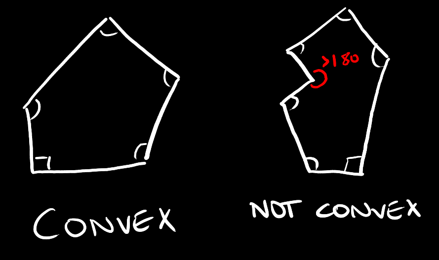
A convex polygon is a polygon whose inner angles are all less than 180 degrees. A hexagon, for example, has all its angles at 120 degrees.

Given a set of points \(Q\) in the plane, given by their \(x\) and \(y\) coordinates, compute the smallest convex polygon \(P\) for which each point in \(Q\) is either on the boundary of \(P\) or in its interior.

Before we begin, let's understand what polar angle is. The polar angle of a point \(p\) with respect to the origin point \(p_0\) is the angle from the x-axis through the origin to the point \(p_0\), rotating counter clockwise.

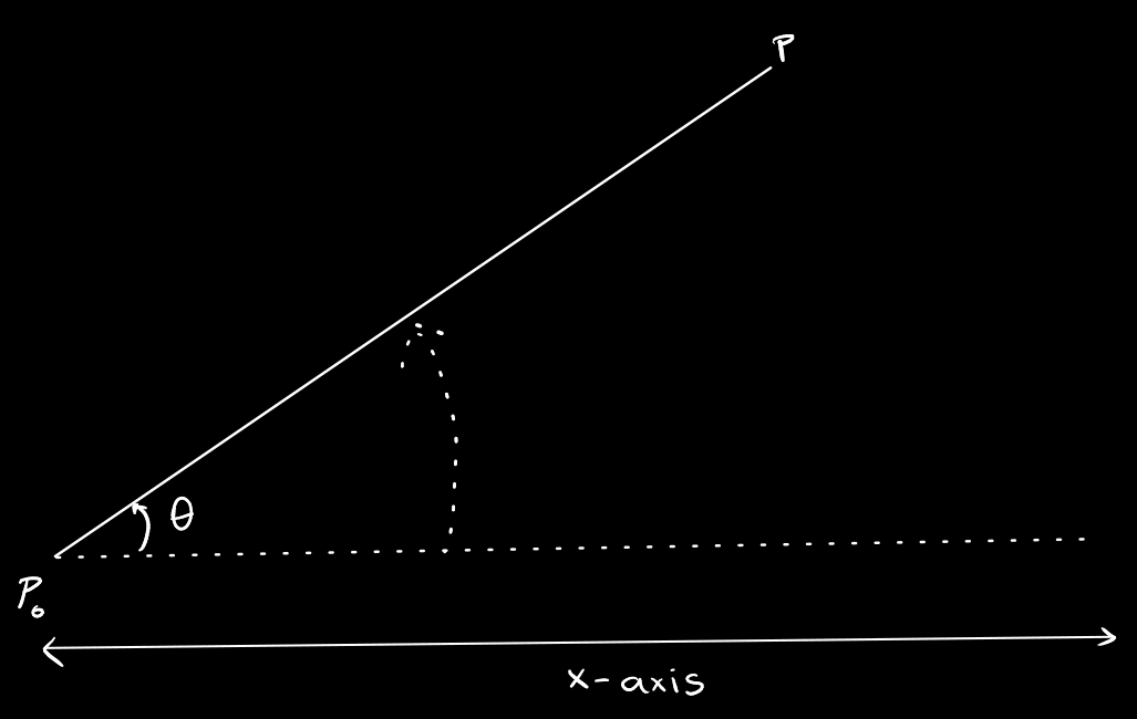
In the above example, \(\Theta\) is the polar angle of \(p\) with respect to \(p_0\).

We can use the following equation to compute the angle formed by three points: \(\Theta: u \cdot v = ||u|| \; ||v|| \cos\Theta\). Here the dot is the dot product of two vectors formed by the points, and \(||u||\) is the length of \(u\).

Note that we cannot assume arccos or square root to be constant-time operations supported by RAM. However, in many algorithms, we just have to compare two angles without computing their actual values. This equation allows us to compare \((\cos\Theta)^2\) in constant time, so we can compare two angles in constant time.

However, instead of comparing the \(\Theta\) values, we can compare the \(\cos(\Theta)\) of the angles to avoid computing arccos. Similarly, we avoid computing the square root by comparing the square of \(\cos{\Theta}\). Since all we need to do is compare values, we can avoid performing extra computation.

A simplifying assumption: No three points are collinear. This is not a hard case to handle but introduces many cases which draw away from the focus of the algorithm.

Brute-Force Solution

Consider the line joined by each pair of points, \(p_1, p_2\). If all the other points are on the same side of this line, then this line must be an edge of our convex hull.

We can test that all other points are on the same side of \(p_1, p_2\) by first determining the equation of the line \(Ax + By + C = 0\). For any other point, substitute the coordinates of the point into the equation. If the signs of all the results are the same, then all the points are on the same side. If the result is 0, then the point is on the line.

We do this for every pair of points to find all the edges of the convex hull.

Running time: \(O(n^3)\)

Jarvis March (Gift-wrapping)

• Start with \(p_0\), the point with the minimum y-coordinate, breaking ties arbitrarily. Assertion: \(p_0\) must be a vertex of the convex hull.

• Find \(p_1\), the point with the smallest polar angle with respect to \(p_0\). This will be the next vertex of the convex hull.

• The next vertex \(p_2\) of the convex hull has the smallest polar angle with respect to \(p_1\). We repeat this process until we get the highest point of the convex hull, say \(p_k\). That would be the point with the maximum value of \(y\).

• Construct the left chain, starting from \(p_k\) and choosing \(p_{k+1}\) as the point with the smallest polar angle with respect to \(p_k\), but from the negative x-axis. We do this until we come all the way back to \(p_0\).

Running time:

Say \(h\) is the number of vertices on the convex hull, then the running time is \(O(nh)\) which in the worst case would be \(O(n^2)\) (all points are on the convex hull).

This algorithm is good if \(h\) is small.

Graham's Scan

This solution uses the ideology of Jarvis March but with the concept of sorting.

• Locate \(p_0\) as the lowest point in \(Q\), breaking ties arbitrarily.

• Sort all other points by polar angle with respect to \(p_0\).

• Process the points starting with the one with the smallest polar angle, scanning the entire list. At each step, compute the convex hull of the points we have already scanned.

• Add each point in turn with the next higher angle.

• If doing so causes a left turn, add the point as a vertex and maintain our convex hull, then continue to the next iteration. Otherwise, if a right turn occurs, the point in the middle of the turn can't be a part of the vertices of the convex hull. Therefore, discard it and join the previous point to the new point and check again.

• This involves a backtracking process, discarding points as we go until we end up making a left turn again.

Pseudocode for backtracking

S ← an empty stack
push(p0, S)
push(p1, S)
push(p2, S)

for i ← 3 to n-1 do

    while (angle between next to top,
        top and pi make non-left turn) do

        pop(s)

    push(pi, S)

return S

For the backtracking, the running time analysis: Each point is visited at most twice. Add it to \(CH(Q)\) and possibly discard it. But once it's been discarded, it's never added to the stack again. Hence it's \(O(n)\) running time.

Therefore, the dominating factor would be \(O(n \lg n)\) from sorting.

Divide And Conquer

The divide and conquer approach breaks down the problem into three parts:

• Divide the given problem into a number of subproblems.
• Conquer the subproblems by solving them recursively.
• Combine the solutions to the subproblems into the solution to the original problem.

The important part is identifying if the solution to subproblems can be used to find the solution to the whole. If you can combine, then you can divide and conquer.

Example: If you have to find the maximum in a given array, and you are given the max of the left half and the max of the right half, can you find the max of the whole? Yes? You can use divide and conquer!

Multiply Two n-bit Non-Negative Numbers

Compute the product of two n-bit non-negative numbers. An array of n entries is used to store the bits in each of these numbers.

If we design an algorithm based on the pencil-and-paper approach, it would require \(O(n^2)\) time. Now let's see if we can make any improvements using divide-and-conquer.

Solution

This suggests a divide-and-conquer algorithm: first, compute the four multiplications in the equation using recursion (each of which is of size n/2). Then, use the solutions to these subproblems to compute XY.

Thus, we have the following recurrence relation on the running time:

Using the iteration approach to solving recursions, we get:

Thus this solution does not achieve any improvement compared to the pencil-and-paper solution.

Karatsuba's Algorithm

This solution is based on the following equation:

If we design a divide-and-conquer approach based on this equation, we only have to solve 3 subproblems: the computation of \(AC\), \((A-B)(D-C)\), and \(BD\). Thus, the running time is reduced to:

Which leads us to:

Since \(\lg 3 = 1.58\dots\), we have \(T(n) = O(n^{1.59})\).

Solving Recurrence Relations

Master Theorem

The Master Theorem can be stated as follows:

Let \(a \geq 1\) and \(b > 1\) be constants. Let \(f(n)\) be a function. Let \(T(n)\) be defined on non-negative integers by the recurrence:

where we interpret \(n/b\) to mean either \(\lfloor n / b \rfloor\) or \(\lceil n/b \rceil\). Then

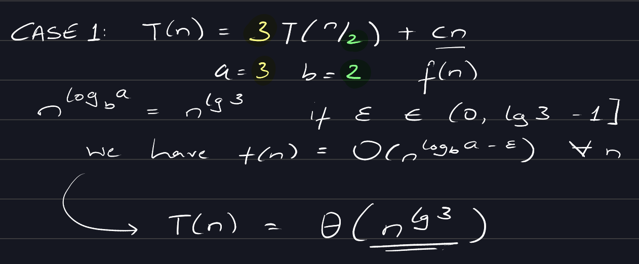
1. If \(f(n) = O(n^{\log_ba-\epsilon})\) for some constant \(\epsilon > 0\), then \(T(n) = \Theta(n^{\log_b a})\).

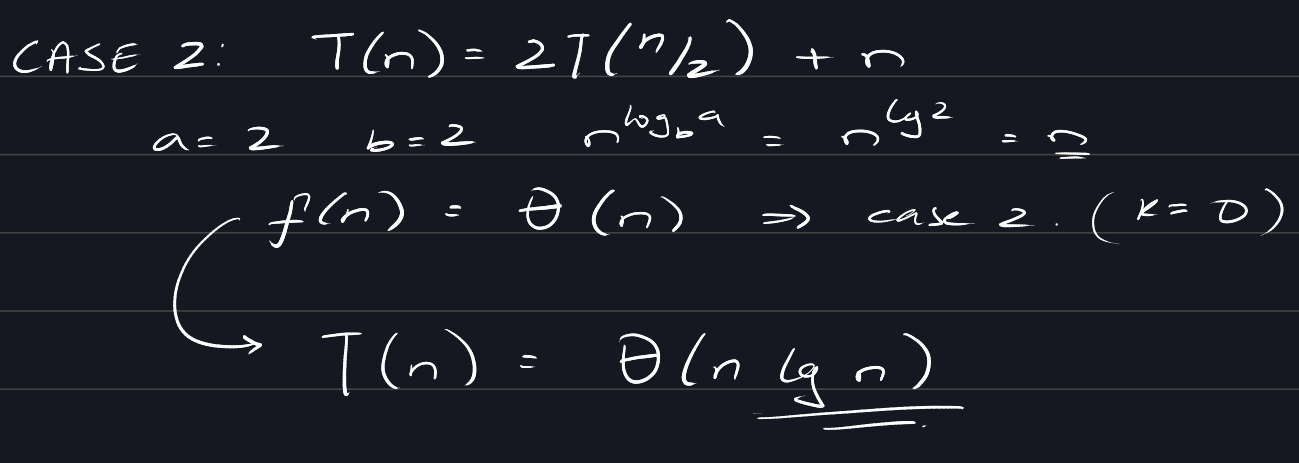
2. If \(f(n) = \Theta(n^{\log_b a} \lg^k n)\) for some constant \(k \geq 0\), then \(T(n) = \Theta(n^{\log_b a} \lg^{k+1} n)\).

3. If \(f(n) = \Omega(n^{\log_b a + \epsilon})\) for some constant \(\epsilon > 0\), and (regularity condition) if \(af(n/b) \leq cf(n)\) for some constant \(c < 1\) and all sufficiently large \(n\), then \(T(n) = \Theta(f(n))\).

Note that this doesn't address all cases.

Examples of each of the cases:

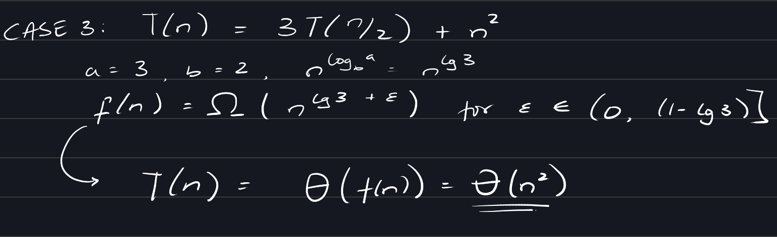
Case 1:

Case 2:

Case 3:

Recursion Tree

In a recursion tree, each node represents the cost of a single subproblem somewhere in the set of recursive function invocations.

Such a tree can be used to calculate the total cost of a function by summing the costs at each layer and identifying how each of the costs changes. The number of layers is also a function of n - hence a recurrence can be solved this way.

We often use a recursion tree to make a good guess, and then prove the guess using the substitution method.

Closest Pair of Points

Find the closest pair of points in a set, \(P\), of \(n\) points.

The distance between two points \((x_1, y_1)\) and \((x_2, y_2)\) can be computed as \(d = \sqrt{( x_1 - x_2 )^2 + ( y_1 - y_2 )^2}\). To compare the distance between one pair of points with the distance between another pair of points, we can compare the square of distances between them to avoid performing the square root operation.

The brute force approach to this will check all pairs of points and thus will require \(\Theta(n^2)\).

Divide-and-Conquer Solution

We split the set \(P\) into two sets \(P_L\) and \(P_R\) of approximately equal size. That is, \(|P_L| = \lceil |P|/2 \rceil\) and \(|P_R| = \lfloor |P|/2 \rfloor\). We do this by first sorting \(P\) by the x-coordinate, and split \(P\) into two with a vertical line \(L\) through the median of the x-coordinates. Thus, \(P_L\) has points on or to the left of \(L\), and \(P_R\) has points on or to the right of \(L\).

We find the closest pair of points in \(P_L\) and \(P_R\) recursively. Let \(\delta_L\) and \(\delta_R\) denote the closest pairs in \(P_L\) and \(P_R\) respectively. Let \(\delta = \min(\delta_L, \delta_R)\).

Now we need to identify if there are points between \(P_L\) and \(P_R\) that are closer than \(\delta\). We observe that if such a point exists, then it must exist within a region around \(L\), being at most \(\delta\) away from it.

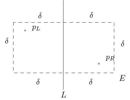
We can also observe there can be at most 4 points in the left half (in the four corners) because if they were any closer then their distance would be shorter than \(\delta\), which should not be possible. Similarly, for the right half.

• Sort the points in the strip of width \(2\delta\) centered at \(L\) by their y-coordinate. We need not consider points that are not in this strip.

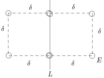
• For these points, compare each of them with 7 following points. This is sufficient for finding \(p_L\) and \(p_R\), since, in the worst case, there are at most 6 points between them from our previous observations.

Speed-up: To avoid sorting for each recursive call, at the beginning of the algorithm, we sort all the points by x-coordinate and store them in an array \(X\). We then sort all the points by y-coordinate and store them in an array \(Y\). With care, we will use these two arrays to avoid sorting in recursive calls.

The content of array \(X\) will not change during the recursive calls. In the divide step, we divide \(X[p..r]\) (the set \(P\)) into \(X[p..q]\) (the set \(P_L\)) and \(X[q+1..r]\) (the set \(P_R\)), where \(q = \left\lfloor \frac{p+r}{2} \right\rfloor\).

When dividing \(P\) into \(P_L\) and \(P_R\), we split \(Y\) into \(Y_L\) and \(Y_R\) by performing a linear scan in \(P\). For each point encountered during this scan, we check whether it is in \(P_L\) or \(P_R\), and copy it to either \(Y_L\) or \(Y_R\) accordingly. We then use \(Y_L\) and \(Y_R\) as arguments for recursive calls.

In the combine step, to sort the points in the strip of width \(2\delta\) centered at \(L\), we perform a linear scan in \(Y\) and extract these points.

The above strategy allows us to perform sorting by x-coordinate once, and by y-coordinate once during the entire execution of the algorithm.

Time Complexity

To analyze the running time, we have the following recurrence relation. Note that the \(O(n \lg n)\) comes from the sorting steps:

We solve this recursion using the master theorem (case 2).

Therefore, the running time of this algorithm is \(O(n \lg^2 n)\).

After the speedup has been applied to the algorithm, thanks to not having to sort inside the recursive call and only performing a linear scan, we get a running time of: \(O(n \lg n)\).

Invent (or Augment) a Data Structure

We use data structures to store data in a particular way to make algorithms faster.

Abelian Square Detection in Strings

In a string, an Abelian square is of the form \(xx'\), where \(|x| = |x'|\) and \(x\) is a permutation of \(x'\). For example, the English word "reappear" is an Abelian square, in which \(x = \text{ reap }\) and \(x' = \text{ pear }\).

The problem we are given provides us with a string \(S[1..n]\) and we have to check if it is an Abelian square in at least one way.

Brute-force Method

We can check if a string is the permutation of another by sorting both strings and then comparing them. Based on this idea, we have the following solution:

for len ← 1 to n/2 do
    for start ← 1 to n - (2*len) + 1 do
        x ← sort(S[start..start+len-1])
        y ← sort(S[start+len..start+2*len-1])
        if (x == y) then
            return true
return false

This has a running time of \(O(n^3 \lg n)\).

Improved Solution

If the strings are defined over a finite alphabet \(\Sigma\) of \(k\) symbols, then we can tell whether \(x\) is a permutation by counting the number of occurrences of each symbol in either string. If each symbol occurs the same number of times in both strings, then \(x\) is a permutation of \(x'\).

To start, we compute a prefix array \(p\) which is a 2D array that stores the number of occurrences of each character up to a given position. \(p[1..k, 0..n]\) holds the count such that \(p[j, m]\) stores the number of occurrences of the letter \(j\) in \(S[1..m]\).

Based on this:

for j ← 1 to k do
    p[j, 0] ← 0

// Compute the prefix 2D array
for i ← 1 to n do
    for j ← 1 to k do
        if S[i] is the j-th letter of the alphabet then
            p[j, i] ← p[j, i-1] + 1
        else
            p[j, i] ← p[j, i-1]

for len ← 1 to n/2 do
    for start ← 1 to n - (2*len) + 1 do
        j ← 1
        while (j ≤ k) and (
            p[j, start+len-1] - p[j, start-1]
            = p[j, start+2len-1] - p[j, start+len-1])

            j ← j + 1

        if j = k + 1
            return true

return false

The running time of this solution is \(O(kn^2)\) where \(k\) is the number of symbols in the alphabet. If \(k\) is not too large, this is much better than the previous solution.

Supporting Subrange Sum Under Updates

We want to maintain an array \(A[1..n]\) to support the following operations:

1. Set \(A[i] \gets A[i] + \delta\)
2. Subrange sum \((c, d)\): Computing \(\sum A[i]\) for all \(i\) from \(c\) to \(d\).

If we simply store the data in the array \(A\), then the first query can be supported in \(O(1)\) time, but the second query requires \(O(n)\) time. Alternatively, if we store the data in the prefix array \(p\), then the second query can be supported in \(O(1)\) time, but the first requires \(O(n)\) time. Now let's design a better data structure.

We can design a tree structure where each node stores the sum of a subarray. Each leaf corresponds to a subarray of length 1, and the level above corresponds to subarrays of length 2, 4, 8, etc.

To support the first query, we simply update \(A[i]\) and all its ancestors, which uses \(O(\lg n)\) time.

To compute the sum of \(A[c..d]\), we compute it as the difference between the sums of \(A[1..d]\) and \(A[1..c]\). To compute the sum of \(A[1..d]\), first initialize a variable named sum to 0. We start from the root and descend to the highest node whose range ends with \(d\), adding its value to sum. During the top-down traversal, each time we choose the right child, we add the value of the left child to the sum.

As the height of this tree is \(O(\lg n)\), the second query can be answered in \(O(\lg n)\) time. Therefore, our data structure can support both queries in logarithmic time.

Greedy Algorithms

The idea behind a greedy algorithm is to make the optimal choice at every step, hoping to reach the global optimal solution. We must find a way of picking the local optimal option such that it leads to the global optimal - this is not the case with all ways we can choose.

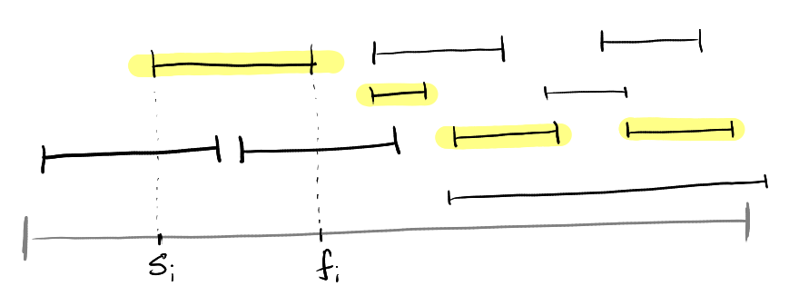
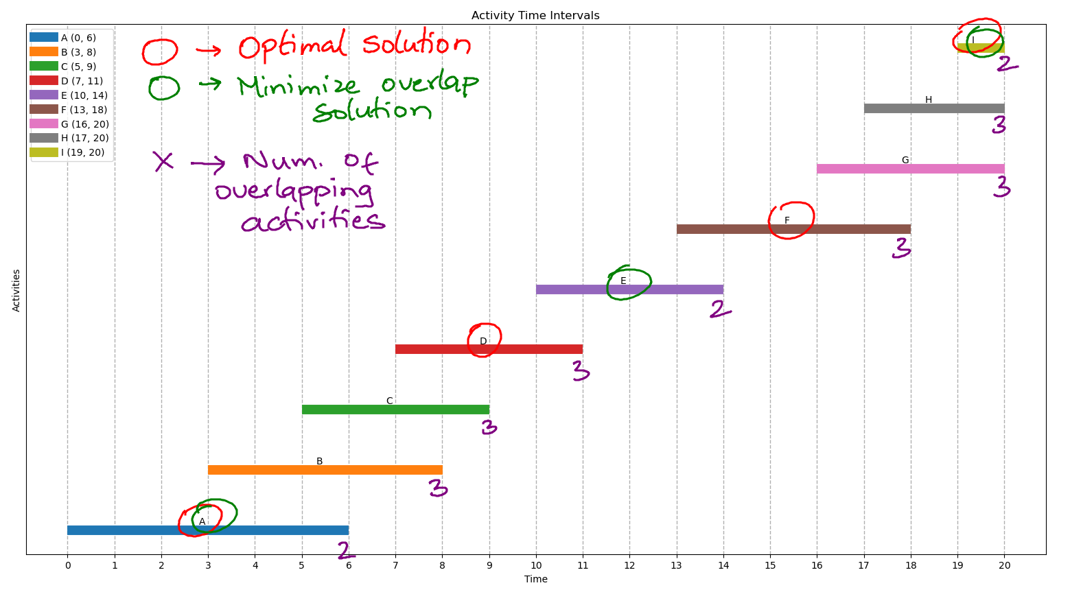
Activity Selection Problem

In this problem, you are given a set of activities competing for time intervals on a given resource. Here \(n\) denotes the number of activities. Each activity has a start time \(s_i\) and a finish time \(f_i\). If selected, activity \(i\) takes up the half-open interval \([s_i, f_i)\).

We are trying to produce a schedule containing the maximum number of compatible activities. We say that activity \(i\) is compatible with activity \(j\) if either \(s_i \geq f_j\) or \(s_j \geq f_i\) holds (they do not overlap).

Greedy strategies that do not work:

• Picking the activity that starts the earliest.
• Picking the shortest activity first.
• Picking the activity that is in the least conflict.

Counterexamples can be generated for each of these strategies. For instance, the situation of picking an activity that is most compatible is proven wrong with this counterexample:

Working Greedy Strategy

The greedy strategy that works for this is always picking the activity that finishes first, i.e., activities that end the earliest.

• Sort activities by finish time in increasing order.
• Start with the first, and choose the next possible activity compatible with the previous ones.

Activity_Selection(s, f, n)
    sort both s and f by f[i] in increasing order
    A ← {1}
    k ← 1
    for i ← 2 to n do
      if s[i] ≥ f[k] then
        A ← A ∪ {i}
        k ← i
    return A

This algorithm has a time complexity of \(O(n \lg n)\).

Correctness

Intuitive Understanding:

Consider an optimal set of activities \((a_1, a_2, \ldots, a_k)\). If we replace \(a_1\) with the first activity of the greedy algorithm, the new set \((1, a_2, \ldots, a_k)\) remains optimal. This is because the first activity finishes at the same time or earlier than \(a_1\), ensuring compatibility with the remaining activities. By repeatedly applying this replacement strategy with \(a_2, \ldots, a_k\) using activities chosen by the greedy algorithm, we transform the optimal solution into the one provided by the algorithm, preserving the activity count.

A more formal proof:

The set of activities selected by the greedy algorithm \((a_1, a_2, \ldots, a_k)\), where each \(a_i\) precedes \(a_{i+1}\) for \(1 \leq i \leq k-1\), is optimal.

Consider an optimal solution \((b_1, b_2, \ldots, b_m)\) with \(b_i\) preceding \(b_{i+1}\) for \(1 \leq i \leq m-1\). We aim to prove \(k = m\).

Inductive Claim: For each \(i\), \(a_i\) finishes no later than \(b_i\).

• Base Case: \(a_1\) ends no later than any other activity.

• Inductive Step: Assume the claim holds for \(i\); we prove it for \(i+1\).

• Define \(S\) as the set of activities compatible with \((a_1, \ldots, a_i)\), and \(S'\) as those compatible with \((b_1, \ldots, b_i)\).
• \(S\) includes activities starting after \(a_i\), and \(S'\) includes those starting after \(b_i\).
• By induction, \(a_i\) finishes no later than \(b_i\), implying \(S' \subseteq S\).
• Since \(b_{i+1} \in S'\), it's also in \(S\).
• By greedy choice, \(a_{i+1}\) finishes earliest in \(S\), so it ends no later than \(b_{i+1}\).

If \(k < m\), activity \(b_{k+1}\) starts after \(a_k\) and is compatible with \((a_1, \ldots, a_k)\). However, the greedy algorithm did not select \(b_{k+1}\) after \(a_k\), which contradicts its compatibility and later finish. Therefore, \(k \geq m\). Since \(k\) cannot be greater than the size of any optimal solution, \(k = m\), proving the optimality of the greedy algorithm's selection.

Knapsack Problem

We have \(n\) items, and each item \(i\) has a weight \(w_i\) (in kg) and a value \(v_i\) (in dollars). We also have a knapsack, which has a maximum weight, \(W\), that it can hold.

We are required to choose items such that we maximize the value we can hold in our knapsack.

There are multiple possible greedy strategies:

1. Most valuable item first
2. Heaviest item first
3. Lightest item first
4. Item with the highest value-to-weight ratio first.

Unfortunately, none of these four strategies works. There are counterexamples that can be presented to prove that each of those does not work.

Therefore, the knapsack problem cannot be solved using a greedy strategy.

Fractional Knapsack Problem

Here, rather than having single physical items, they represent some items that can be partitioned into smaller chunks (such as sugar or sand).

Thus, we can take a fraction of an item and put it into our knapsack.

Under these assumptions, the greedy strategy of picking the items with the highest value-to-weight ratio works. This is because we can take a fractional amount of the final item to max out our knapsack's weight.

greedy(n, v, w, W)
    sort both v and w by the ratio v[i]/w[i] in decreasing order
    free ← W
    sum ← 0
    for i ← 1 to n do
      x ← min(w[i], free)
      sum ← sum + v[i] * (x/w[i])
      free ← free - x
    return sum

Correctness

This proof demonstrates the optimality of the greedy solution for the knapsack problem through contradiction. We consider two cases: where the ratio of value to weight \(\frac{v[i]}{w[i]}\) for each item is distinct, and where they are not necessarily distinct.

Case 1: Distinct Value-to-Weight Ratios

We start off with our assumption:

Suppose an optimal solution \(S\) surpasses our greedy solution \(G\). Both solutions initially agree on a set of items and then diverge.

We use proof by contradiction:

1. Items are ordered by \(\frac{v[i]}{w[i]}\) in decreasing order.
2. Let \(k\) be the first item where \(S\) and \(G\) choose different amounts.
3. Greedy solution \(G\) selects the maximum amount of item \(k\) that fits, say \(g\) kg.
4. Optimal solution \(S\) picks less of item \(k\), say \(s\) kg.

Contradiction: We can swap \((g - s)\) kg of later items in \(S\) with an equal weight of item \(k\). This exchange increases the total value of \(S\), contradicting the assumption of its optimality.

Case 2: Non-Distinct Value-to-Weight Ratios

For items with the same \(\frac{v[i]}{w[i]}\) ratio, group them together. Then apply the same reasoning as in Case 1.

Egyptian Fractions

Egyptian fractions date back almost 4000 years to the Middle Kingdom of Egypt. They take the form \(\frac{1}{x_1} + \frac{1}{x_2} + \ldots + \frac{1}{x_n}\), where each \(x_i\) is a distinct positive integer, representing a sum of unit fractions. For instance:

• \(\frac{5}{6} = \frac{1}{2} + \frac{1}{3}\)
• \(\frac{47}{72} = \frac{1}{2} + \frac{1}{9} + \frac{1}{24}\)

These fractions were practical for ancient Egyptians in everyday calculations. For example, to distribute 47 sacks of grain evenly among 72 farmhands, a farmer would use the equation \(\frac{47}{72}\) as an Egyptian fraction. This involved:

1. Giving each person \(\frac{1}{2}\) of a sack from 36 sacks.
2. Distributing \(\frac{1}{9}\) of a sack from 8 sacks.
3. Allocating \(\frac{1}{24}\) of a sack from the remaining 3 sacks.

Thus, each person received \(\frac{1}{2} + \frac{1}{9} + \frac{1}{24} = \frac{47}{72}\) of a sack, achieving a fair division.

Fibonacci's Greedy Approach in 1202

In 1202, Fibonacci introduced a greedy method to express any rational number as a sum of unit fractions. This approach is based on the equation:

To validate this, consider:

Applying this method repeatedly yields unit fractions, with the numerator of the second term decreasing until the algorithm terminates. For example, \(\frac{47}{72}\) using Fibonacci's method is:

This demonstrates that the greedy expansion is not always the shortest or the one with the smallest denominator.

Open Problem: Egyptian Fraction Representation of 4/n

A current open problem challenges the claim that every fraction of the form \(\frac{4}{n}\), where \(n\) is an odd integer, can be expressed as an Egyptian fraction with exactly three terms.

Dynamic Programming

Dynamic programming was popularized by Richard Bellman. This algorithmic paradigm usually applies to optimization problems. It typically reduces the complexity from exponential (e.g., \(2^n\)) to polynomial, e.g., \(O(n^3)\). This is achieved by avoiding the enumeration of all possibilities.

Dynamic programming usually involves storing intermediate results to prevent re-computation. It also involves having multiple cases and deciding on a particular case for the optimal solution. A greedy strategy doesn't work because there are more than one cases.

Matrix-Chain Multiplication

The way we multiply a matrix is by taking the dot product of the row vectors from the left matrix and the column vectors from the right matrix. Consider the matrices \(A\) of dimensions \(n \times p\) and \(B\) of dimensions \(p \times m\). Note that the number of columns of the first and the number of rows of the second need to match.

The number of scalar multiplications in such a computation would be \(m*p*n\).

Now consider the multiplication of more than one matrix. The order in which we compute the multiplication greatly changes the number of operations required.

Consider the following three matrices:

• \(M_1\): \(10 \times 100\)
• \(M_2\): \(100 \times 5\)
• \(M_3\): \(5 \times 50\)

There are two ways of computing \(M_1 * M_2 * M_3\). If we compute it as \(M_1(M_2M_3)\), the number of scalar multiplications is \(75,000\). If we compute it as \((M_1 M_2) M_3\), the number of scalar multiplications is \(7,500\). The difference is a factor of 10!

Our problem is going to be finding the sequence of multiplications that leads to the fewest number of scalar multiplications given a number of matrices.

Brute Force Solution

We could use a brute-force approach, trying all possibilities and taking the minimum. The running time depends on the total number of ways to multiply \(n\) matrices. Let \(W(n)\) denote this number.

To compute \(W(n)\), we make use of the observation that the last multiplication is either \(M_1 (M_2 ... M_n)\) or \((M_1 M_2)(M_3 ... M_n)\), and so on until \((M_1...M_{n-1})M_n\).

From this observation, we can conclude that \(W(n) = 1\) if \(n = 1\), and \(W(n) = \sum W(k) * W(n-k)\).

Then we can prove that:

From this, we get that the order of this is \(W(n) \approx 4^n/(n^{3/2})\), which is exponential.

Dynamic Programming Approach

We use dynamic programming to store the intermediate results to avoid re-computation in a recursive approach, thus achieving a polynomial time solution.

We make use of the following observation: Suppose the optimal method to compute the product \((M_1M_2...M_n)\) was to first compute the product of \(M_1M_2...M_k\) (in some order), then compute \(M_{k+1}M_{k+2}...M_n\) (in some order), and then multiply these two results together. Then the method used for the computation of \(M_1M_2...M_k\) MUST BE OPTIMAL, for otherwise, we could substitute a better method to compute \(M_1M_2...M_k\), thereby improving the optimal method for \(M_1M_2...M_n\). Similarly, the method used to compute \(M_{k+1}M_{k+2}...M_n\) must also be optimal. What remains is to find the value of \(k\), and there are \(n-1\) choices.

Based on this, we further develop our algorithm. Let \(m[i, j]\) be the optimal cost for computing \(M_iM_{i+1}...M_j\). Then we have

This can be translated to a recursive algorithm. However, this is an extremely slow algorithm because it performs a lot of re-computation.

Recursive_Multi(i, j)
  if i = j then
    return 0
  else
    minc ← ∞
    for k ← i to j-1 do
      a ← Recursive_Multi(i, k)
      b ← Recursive_Multi(k+1, j)
      minc ← min(minc, a+b+p[i-1]*p[k]*p[j])
  return minc

This algorithm checks all possibilities and, therefore, is as bad as the brute-force solution.

To use dynamic programming, we fix an order in which we compute \(m[i, j]\). Here we first compute \(m[i, i]\) for all \(i\). Then we compute \(m[i, i+1]\) for all \(i\), and so on.

Matrix_Multi_Order(p, n)
  for i ← 1 to n do
    m[i,i] ← 0

  for d ← 1 to n-1 do
    for i ← 1 to n-d do
      j ← i + d
      m[i,j] ← ∞
      for k ← i to j-1 do
        q ← m[i,k] + m[k+1,j] + p[i-1]*p[k]*p[j]
        if q < m[i,j] then
          m[i,j] ← q
          s[i,j] ← k
  return (m, s)

The running time of this algorithm is \(O(n^3)\), and the optimal cost of multiplying these matrices is stored in \(m[1, n]\).

Say we wish to multiply \(M_i * M_{i+1} * \dots M_j\) optimally, if we know \(k\), then we can compute \(M_i * M_{i+1} \dots M_k\) and \(M_{k+1} * M_{k+2} \dots M_j\) recursively, and then multiply the products together.

Matrix_Mult(M, s, i, j)
  if j > i then
    X ← Matrix_Mult(M, s, i, s[i,j])
    Y ← Matrix_Mult(M, s, s[i,j]+1, j)
    return X*Y
  else
    return Mi

The cost of this multiplication is \(O(n) +\) the cost of the actual multiplication of the matrices.

Memoization Approach

Another approach is to use the previously mentioned recursive algorithm, using memoization to store intermediate results to prevent re-computation.

Memoized_Matrix_Multi(p, n)
  for i ← 1 to n do
    for j ← 1 to n do
      m[i,j] ← ∞
  return Lookup(p, 1, n)

Lookup(p, i, j)
  if m[i,j] < ∞ then
    return m[i,j]

  if i = j then
    m[i,j] ← 0

  else
    for k ← i to j-1 do
      q ← Lookup(p, i, k) + Lookup(p, k+1, j) + p[i-1]*p[k]*p[j]
      if q < m[i,j] then
        m[i,j] ← q
        s[i,j] ← k

  return m[i,j]

The running time of this memoized algorithm is also \(O(n^3)\).

Longest Common Subsequence

We are given two strings \(x[1..m]\) and \(y[1..n]\), and our task is to find the longest sequence that appears (not necessarily consecutively) in both strings.

For example, if x = "algorithm" and y = "exploration", then their LCS (longest common subsequence) is "lort".

If we solve this problem using a brute-force approach, by enumerating all possible subsequences of \(x\) and \(y\) and then computing their intersection, the running time would be exponential.

Solution

Consider the last character of either string. There are three cases:

1. If \(x[m] = y[n] = a\), then any longest common subsequence, \(z[1..k]\), of \(x\) and \(y\) will end in \(z[k] = a\) (otherwise, we can append it to get a longer sequence). It's also the case that \(z[1..k-1]\) is a longest common subsequence of \(x[1..m-1]\) and \(y[1..n-1]\).

2. If \(x[m] \neq y[n]\), then \(z[k] \neq x[m]\), also \(z[1..k]\) is a longest common subsequence of \(x[1..m-1]\) and \(y[1..n]\).

3. If \(x[m] \neq y[n]\), then if \(z[k] \neq y[n]\), that implies that \(z[1..k]\) is the longest common subsequence of \(x[1..m]\) and \(y[1..n-1]\).

Let \(c[i,j]\) be the length of the LCS of these two prefixes: \(x[1..i]\) and \(y[1..j]\). Then, based on the above observation, we have:

Then we can use the following algorithm to compute all the entries of \(c\), and return the length of LCS \(x\) and \(y\).

LCS_Length(x[1..m], y[1..n])
  for i ← 1 to m do
    c[i,0] ← 0

  for j ← 1 to n do
    c[0,j] ← 0

  for i ← 1 to m do
    for j ← 1 to n do
      if x[i] = y[j] then
        c[i,j] ← c[i-1, j-1] + 1
      else
        c[i,j] ← max(c[i-1,j], c[i,j-1])

  return c[m,n]

To compute the actual LCS of the strings, we can use the following function:

LCS(i, j)
  if i = 0 or j = 0 then
    return empty string

  else if c[i,j] > max(c[i-1,j], c[i,j-1]) then
    return (LCS(i-1,j-1), x[i])
  else if c[i-1,j] >= c[i,j-1] then
    return LCS(i-1,j)
  else
    return LCS(i,j-1)

The running time of the \(LCS(m,n)\), observes that each call decreases the value of \(i, j\) or both by \(1\). Therefore, the number of calls is at most the sum of the initial values of \(i\) and \(j\), which is \(m+n\). The work in each call costs constant time, so the total running time is \(O(m+n)\).

Making Change Problem

In this problem, we are given an amount in cents. We are to make change using a system of denominations, using the smallest number of coins possible to make change.

We can think of using a greedy algorithm to choose as many highest value coins as possible and reduce to a lower value once we can't take any more. However, this does not work for all possible coinage systems.

Solution

To use dynamic programming for the problem of making change, we assume in the input we have the amount (in cents) \(n > 0\), and an array \(d[1..k]\) storing the denominations of the \(k\) coins, in which \(d[1] = 1\) (so that we can always make exact change) and \(d[i] < d[i+1]\) for all \(i\).

We make the following observation: The optimal method must use some denomination \(d[i]\). If we know which \(d[i]\) is used, then we can claim that the optimal solution can be computed by first computing the optimal solution for \(n-d[i]\), and then adding one coin of denomination \(d[i]\). We do not know which coin is to be used, so we try all \(d[i]\) such that \(d[i] \leq n\).

This gives us the following recursion, in which \(\text{opt}[j]\) stores the optimal number of coins to make change for \(j\) cents.

We can then write an algorithm to compute \(\text{opt}[j]\) for \(j = 1, 2, \ldots, n\).

Coins(n, d[1..k])
  for j ← 1 to n do
    opt[j] ← ∞

    for i ← k downto 1 do

      if d[i] = j then
        opt[j] ← 1
        largest[j] ← d[i]

      else if d[i] < j then
        a ← 1 + opt[j-d[i]]
        if a < opt[j] then
          opt[j] ← a
          largest[j] ← d[i]
  return opt[n]

The running time is \(O(kn)\).

Let's look at an example. In this example, \(d = \{1, 4, 5\}\). Then, the greedy algorithm would express 8 as 5+1+1+1 and uses 4 coins. If we use dynamic programming, we will compute the entries of opt and largest as follows:

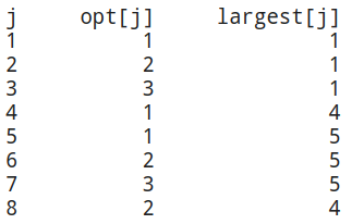
Based on the above process, we can design an algorithm that will compute the set of coins used in the optimal solution, assuming that the array largest has already been computed using dynamic programming.

Make_Change(n, largest)
  C ← Φ   // a multiset that stores the answer
  while n > 0 do
    C ← C ∪ largest[n]
    n ← n - largest[n]
  return C

Exploiting The Problem's Structure

Many problems have some sort of structure (algebraic, number-theoretic, topological, geometric, etc.) that suggests a solution, so we design algorithms accordingly to make use of such structure.

Greatest Common Divisor

Given non-negative integers \(u\) and \(v\), compute their greatest common divisor, \(gcd(u, v)\).

The brute-force approach (trying all possible numbers) is going to take a running time of \(O(\min(u, v))\). However, this is not linear time if the numbers are large enough and the divisibility operation takes more than constant time.

If the numbers are stored in \(\lg u\) bits then the running time would be \(O(u)\) which would be approximately \(O(2^{\text{input size}/ 2})\), which would be exponential time.

Euclid's Algorithm

If \(d \mid u\) and \(d \mid v\), then \(d \mid (au + bv)\) for all integers \(a\) and \(b\). We then choose \(a=1\) and \(b=-\lfloor u/v \rfloor\) and then

From this, we get Euclid's algorithm:

Euclid(u, v)
    while (v ≠ 0) do
        (u, v) ← (v, u mod v)
    return u

Finch proved that this algorithm takes \(O(\lg n)\) time on a given input where \(u > v > 0\). This means that Euclid's algorithm is linear in time (for large numbers).

Binary Algorithm

The binary algorithm avoids using integer division and uses subtraction and shifts instead. Its running time does not beat that of Euclid's algorithm asymptotically. However, in practice, it often uses less time as subtraction/shift are faster than division. It was proposed by J. Stein in 1967, though an approach used in the 1st century of China is essentially equivalent. Here, we use Stein's modern description.

This algorithm is based on the following recurrence, in which \(u \geq v\):

From this, we get the following pseudocode:

GCD(u, v)
  if u < v then
    return GCD(v, u)
  if v = 0 then
    return u
  if u and v are both even then
    return 2*GCD(u/2, v/2)
  if u is odd and v is even then
    return GCD(u, v/2)
  if u is even and v is odd then
    return GCD(u/2, v)
  return GCD((u-v)/2, v)

This algorithm has a running time of \(O(\max(\lg u, \lg v))\).

Probabilistic And Randomized Techniques

In probabilistic analysis, we use knowledge of, or make assumptions about, the distribution of input. We average the running time over the distribution of possible inputs to get the average-case running time. One classic example is quicksort!

Randomized algorithms are determined by input and by values produced by a random-number generator.

Majority Element Problem

We are given an array \(A[1..n]\) of integers, in which one integer (the majority element) occurs more than \(n/2\) times, and our task is to find this element. This problem has applications in data mining.

The following is a simple randomized algorithm for this problem:

Find_Majority(A[1..n])
  while true do
    i ← RANDOM(1, n)
    Get the number, j, of occurrences of A[i] in A[1..n]
    if j > n/2 then
      return A[i]

To get the expected running time, we first observe that since there is a majority element, the probability of finding it in one try (i.e., one iteration of the while loop) is greater than 1/2. Thus, the expected number of tries to find it is less than 2 (proved later). Each try uses \(O(n)\) time, and thus the expected running time is \(O(2n)\).

To analyze the expected number of tries, let's brush up some knowledge in probability theory. The expectation of a random variable \(X\) that can take any of the values in a set \(S\) is

For example, when we toss a die, if the die is fair, the expected value of the die is

Now let's analyze the expected number of tries. In each try, we guess an index of the array, and we find the majority with probability \(p > \frac{1}{2}\). (Here \(p\) is equal to the number of occurrences of the majority divided by \(n\).) Let \(x\) be the expected number of tries. Then

We have

Plugging in the value of \(y\), we have \(x \cdot (1-p) + (1-p) = x - p\). Solving this equation, we have \(x = 1/p\). This is indeed less than 2.

So far, we have shown that the above randomized algorithm uses \(O(n)\) expected time, which is efficient. However, there are some issues with this solution. First, this solution is not robust: If there is no majority element, it will loop forever. For some applications, this issue can be resolved by terminating the while loop after a certain number of iterations. If no majority element has been found, then we can claim that, if there is indeed a majority element, then the probability of our algorithm not finding it is less than some threshold. This is acceptable in many applications in data mining, but may not always be acceptable. Another issue is that it may take a long time, though this is rare.

There indeed exists a deterministic algorithm that can solve this problem in \(O(n)\) time. This is the Boyer-Moore's voting algorithm. It is a subtle algorithm. If you are interested, you can read the following optional reading material: utexas source.

Graph Algorithms

A graph is a discrete structure. It is an abstract representation of a set of objects where some pairs of objects are connected by links. We call each object a vertex or node, and each link an edge. Thus, formally, a graph \(G\) can be defined as a pair \((V, E)\), in which \(V\) is the set of vertices, and \(E\) is a set of edges. \(E\) is a subset of \(V \times V\).

Definitions

• In a directed graph, each edge has a direction. When we draw a directed graph, we use arrows to orient edges, showing the direction. We say that edge \((u, v)\) is incident from (leaves) vertex \(u\) and is incident to (enters) vertex \(v\). Simply, edge \((u, v)\) is from \(u\) to \(v\).

• In an undirected graph, edges do not have directions. Edge \((u, v)\) is incident on \(u\) and \(v\). We say vertex \(u\) is adjacent to \(v\) if \((u, v)\) is in \(E\).

• A weighted graph assigns a weight to each edge.

• The degree of a vertex in an undirected graph is the number of edges incident on it. In a directed graph, the in-degree of a vertex is the number of edges entering it, and its out-degree is the number of edges leaving it.

• A loop, or self-loop, is an edge from a vertex to itself. A multi-edge is two or more edges incident to the same pair of vertices. A simple graph is a graph that has no loops or multi-edges.

• A path is a series of vertices in which each vertex is connected to the previous vertex by an edge. The length of a path is the number of edges in the path. A simple path is a path without repeated vertices or edges.

• A cycle is a path whose first vertex is the same as the last vertex. A cycle is simple if, except for the repetition of the start and end vertices, there are no repeated vertices or edges.

• An undirected graph is connected if there is a path between any two vertices.

• A tree is a special type of graph. It is a connected, acyclic graph. If we pick one node of the tree as the root, it is a rooted tree. If not, it is an unrooted tree.

Representations

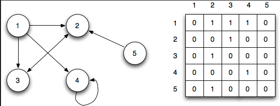
Matrix Representation: In the adjacency matrix representation, we represent a graph \(G = (V, E)\) as a \(|V| \times |V|\) matrix, say \(A\), where \(A[i, j] = 1\) if \((i, j)\) is in \(E\), and \(A[i, j] = 0\) otherwise.

Here is an example:

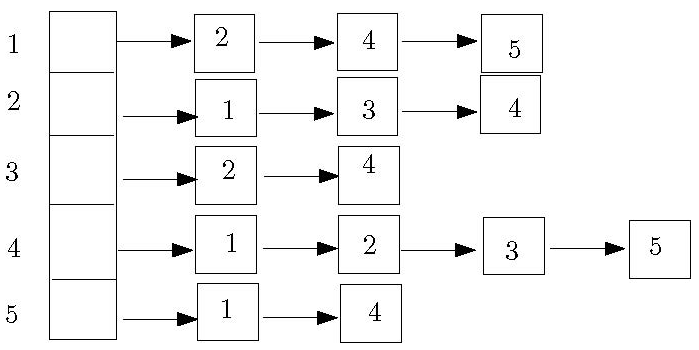
The adjacency list represents a graph as an array, \(Adj[1..|V|]\), of lists. \(Adj[u]\) is a list that contains all the vertices \(v\) such that \((u, v)\) is in \(E\).

Example of an adjacency list:

Minimum Spanning Trees

A spanning tree is an unrooted tree that connects all the vertices of a connected, undirected graph. Every connected graph has at least one spanning tree. If there are weights on edges, the minimum spanning tree (MST) is a spanning tree that minimizes the sum of the weights of the edges used.

Kruskal's Algorithm

In Kruskal's algorithm, at each step, we choose the minimum-weight edge that does not create a cycle. More precisely, in this algorithm, we work with the following two sets:

• A forest (i.e., a set of trees). Initially, each vertex of the graph is a tree by itself in this forest.

• A set of edges \(E'\). Initially, \(E' = E\).

At each step, we remove and consider a minimum-weight edge from \(E'\), breaking ties arbitrarily. If this edge connects two different trees in the forest, then add it to the forest, joining two trees. Otherwise, it connects two vertices from the same tree, forming a cycle. In this case, we discard this edge. When \(E'\) is empty, the forest becomes an MST.

Correctness

First, we prove that the algorithm produces a spanning tree. The resulting graph produced by Kruskal's algorithm cannot have a cycle because if it did, the edge added that forms the cycle would join together two vertices in the same tree, and this is not possible by the algorithm.

The resulting graph must be connected; if it weren't, when we considered the edge that connected two components, we would have added it, but we didn't.

Now we prove that the spanning tree, \(T\), produced by Kruskal's algorithm is minimum. Here we give a proof by contradiction:

Assume to the contrary that \(T\) is not an MST. Among all the MSTs of the graph \(G\), let \(T'\) be the one that shares the largest number of edges with \(T\). Consider the edge \(e\) in \(T - T'\) that was the first edge added to \(T\) by the algorithm.

Because \(T'\) is a spanning tree, adding \(e\) into \(T'\) would create a cycle. Let \(C\) be the cycle in \(T' \cup \{e\}\). Since \(T\) is a tree, it cannot contain all the edges in \(C\). Let \(f\) be an edge in \(C\) that is not in \(T\).

Now consider \(T'' = (T' \cup \{e\}) - \{f\}\), i.e., the tree obtained from \(T'\) by adding edge \(e\) and removing edge \(f\). \(T''\) is also a spanning tree. Since \(T'\) is minimum, we have \(\text{weight}(e) \geq \text{weight}(f)\), for otherwise, \(T''\) would have a smaller total weight than \(T'\), which contradicts the assumption that \(T'\) is the MST that shares the largest number of edges with \(T\).

If \(\text{weight}(f) < \text{weight}(e)\), then Kruskal's algorithm would have considered edge \(f\) before edge \(e\). As \(e\) was the first edge of \(T\) that is not in \(T'\), all the edges added before \(f\) are also in \(T'\). Since \(f\) is in \(T'\), adding it would not create a cycle. Thus Kruskal's algorithm would have added \(f\). As \(f\) was not added, this means \(\text{weight}(f) \geq \text{weight}(e)\).

Therefore, \(\text{weight}(f) = \text{weight}(e)\). Thus the total weight of \(T''\) is equal to the total weight of \(T'\), which means that \(T''\) is also an MST. We also observe that \(T''\) shares one more edge with \(T\) than \(T'\) does, which contradicts the assumption.

Implementation

We must first sort the edges by weight. When considering an edge \((u, v)\), we need to augment another data structure to decide whether they are in the same tree.

If we treat each tree in the forest as a set of vertices, we can abstract the problem of implementing Kruskal's algorithm and define a data structure problem called the disjoint-set data structure problem. Our disjoint sets need to support the following operations:

• MAKE-SET: Create a set containing a single vertex.
• FIND: Given a vertex, find the name of the set it is in.
• UNION: Union together two sets.

This is also called the "union-find" problem.

If we assume we have a data structure solution to the union-find problem, then we can use it to implement Kruskal's algorithm.

// G: Graph (V, E) and w is a weight function.
Kruskal(G, w)
  A ← Φ
  for each v in V do
    MAKE-SET(v)

  Sort the edges of E by increasing order of weight

  for each edge(u, v) in E in increasing order of weight do
    if FIND(u) ≠ FIND(v) then
      A ← A ∪ {(u, v)}
      UNION(u, v)

  return A

Linked List Union-Find

One solution to the problem of Union-Set is representing each set as a linked list of vertices. The name of each set is the first element in its list. For each set, we also maintain a tail pointer that points to the end of the list, and a number field which records the number of elements in the list. Each element in the list stores two pointers: one to the next element, and the other to the head of the list.

With the above structure, it is easy to support the MAKE-SET and FIND in \(O(1)\) time. To support UNION(u, v), we perform the following steps:

1. Follow the head pointer of \(u\) to its head. Follow the head pointer of \(v\) to its head.

2. From the number field, we can tell which list is smaller. Assume without loss of generality that \(u\) is the smaller list. We link \(u\)'s list to the end of \(v\)'s list.

3. Traverse \(u\)'s list, updating head pointers.

4. Update the number field and tail pointer of \(v\)'s list.

The above process uses \(O(t)\) time, where \(t\) is the size of the smaller list.

Time Complexity

To analyze the running time, we can tell that we called the UNION \(n-1\) times to union \(n\) sets (the initial size of each set is 1). In each union, the smaller list becomes part of a list of at least twice the size. Therefore, an element's head pointer is updated at most \(O(\lg n)\) times during all the \(n\) operations. Thus \(n-1\) UNION operations use \(O(n \lg n)\) time in total.

The total running time of Kruskal's algorithm is \(O(|E| \lg |E|)\), which is also \(O(|E| \lg |V|)\), as \(|V| < |E|^2\).

Prim's Algorithm

This is a greedy strategy to solve the MST problem. At each step, choose a previously unconnected vertex that becomes connected by a lowest-weight edge. More precisely, we work with a set of vertices \(V'\), which initially contains an initial vertex arbitrarily chosen. We also work with a set of edges \(E'\), which is initially empty. At each step of the algorithm, we choose an edge \((u, v)\) of minimal weight with \(u \in V'\) and \(v \notin V'\), breaking ties arbitrarily. We add \(v\) to \(V'\) and \((u, v)\) to \(E'\). When \(V' = V\), \(E'\) becomes the MST.

From this description, we see that Prim's algorithm "grows" a tree into an MST, while Kruskal's algorithm merges a set of trees into an MST.

Implementation

At each step, we pick a vertex \(v \notin V\) and this vertex has the minimum-cost edge connecting \(v\) to some vertex in \(V'\). Therefore, a priority queue would be perfect. A priority queue can be implemented using a heap.

For each vertex \(u\), we set its key, \(key[u]\), to be the weight of the minimum-cost edge connecting \(u\) to some vertex in \(V'\), and maintain the vertices not in \(V'\) in a heap structure.

We require the following operations:

• EXTRACT-MIN: removes the element with the minimum key value from the heap and returns it.

• DECREASE-KEY: decrease the key value of a given element.

Both operations can be supported in \(O(\lg n)\) time, where \(n\) is the number of elements in the heap.

// r is the initial vertex / root of MST to be computed
PRIM(G, w, r)
  for each vertex u in V do
    key[u] ← ∞
    π[u] ← NULL

  key[r] ← 0

  // build a heap containing all the vertices in Q
  Q ← V

  while Q ≠ Φ do
    u ← EXTRACT-MIN(Q)

    // Adj is the adjacency list representation of G
    for each v in Adj[u] do
      if v in Q and w(u,v) < key[v]
        π[v] ← u
        key[v] ← w(u,v)  // DECREASE-KEY is used here

We maintain a flag for each vertex \(v\) to check if \(v \in Q\).

Time Complexity

This algorithm has a time complexity of \(O(|E| \lg |V|)\), which matches the running time of Kruskal's algorithm.

If we use Fibonacci heaps (instead of the standard binary heap) to implement Prim's algorithm, we can improve its running time to \(O(|E| + |V| \lg |V|)\).

Single-Source Shortest Path

In a weighted, directed graph, the shortest path from a vertex \(s\) to another vertex \(v\) is a sequence of directed edges from \(s\) to \(v\) with the smallest total weight.

We are given a source and need to find the shortest path to a destination vertex \(v\). For most known algorithms, it is as efficient to find the shortest path from \(s\) to all other vertices of the graph, so we'll just compute the shortest paths to all vertices from \(s\).

In the case where we have edges with negative weights such that there is a cycle with a negative weight, a shortest path from \(s\) to another vertex may not exist. If there is a negative-weight cycle, we are required to detect it.

Before we begin, we will use the following data structures in our solutions:

1. An array \(\pi[1..|V|]\) in which \(\pi[v]\) stores the predecessor of \(v\) along a path.

2. A shortest-path estimate array \(d[1..|V|]\), in which \(d[v]\) stores the current upper bound on the weight of the shortest path from \(s\) to \(v\).

The following will be used to initialize the arrays:

INITIALIZE(G, s)
  for each vertex v in V do
    d[v] ← ∞
    π[v] ← NULL
  d[s] ← 0

One key operation used in the two algorithms that we will learn is the relaxation of the edges. In this operation, we have shortest path estimates to two vertices, \(u\) and \(v\). Then we consider an edge \((u, v)\) to update our estimate on \(v\). The following is the pseudocode:

RELAX(u, v, w)
  t ← d[u] + w(u, v)

  if d[v] > t then
    d[v] ← t
    π[v] ← u

Bellman-Ford Algorithm

The Bellman-Ford algorithm solves the problem in the general case in which edge weights may be negative. When there is a reachable negative-weight cycle, it returns false.

The algorithm essentially uses a loop to keep performing RELAX on all edges. Later we will prove that it is sufficient to iterate this loop \(|V|-1\) times.

BELLMAN-FORD(G, w, s)
  INITIALIZE(G, s)

  for i ← 1 to |V|-1 do
    for each edge (u, v) in E do
      RELAX(u, v, w)

  for each edge (u, v) in E do
    if d[v] > d[u] + w(u, v) then
      return false

  return true

The last for-loop in the above pseudocode performs the negative cycle detection by determining whether we can further update the estimates using RELAX on all edges. It is easy to see that this algorithm uses \(O(|V||E|)\) time.

Correctness

In the first step, we prove the following lemma: After \(i\) iterations of the first "for" loop, the following properties hold:

1. If \(d[v] < \infty\), then \(d[v]\) stores the weight of some path from \(s\) to \(v\).

2. If there is a path from \(s\) to \(v\) with at most \(i\) edges, then \(d[v]\) is less than or equal to the weight of the shortest path from \(s\) to \(v\) having at most \(i\) edges.

(Why do we need this lemma? Consider: What is the maximum number of edges in a simple path? The answer is \(|V|-1\). Thus, when \(i = |V|-1\), the algorithm has considered all simple paths, and from the two properties above, we can claim that, if there is no negative-weight cycle, \(d[v]\) would store the weight of the shortest path from \(s\) to \(v\) after the first "for" loop.)

Proof

We prove by induction on \(i\).

In the base case, \(i = 0\). Before the first "for" loop, \(d[s] = 0\), which is correct. For any other vertex \(u\), \(d[u] = \infty\), which is also correct, as there is no path from \(s\) to \(u\) using 0 edges.

Assume the claim is true for \(i-1\); we now prove it for \(i\).

To prove property 1, consider when a vertex \(v\)'s estimated distance is updated by \(d[u] + w(u, v)\). By our induction hypothesis, \(d[u]\) is the weight of some path, \(p\), from \(s\) to \(u\). Then \(d[u] + w(u, v)\) is the weight of the path that follows \(p\) from \(s\) to \(u\), and then follows a single edge to \(v\).

To prove property 2, consider the shortest path \(q\) from \(s\) to \(v\) with at most \(i\) edges. Let \(u\) be the last vertex before \(v\) on \(q\). Then the part of \(q\) from \(s\) to \(u\) is the shortest path from \(s\) to \(u\) with at most \(i-1\) edges. By the induction hypothesis, \(d[u]\) after \(i-1\) iterations of the 1st "for" loop is less than or equal to the weight of this path. Therefore, \(d[u] + w(u, v)\) is less than or equal to the weight of \(q\). In the \(i\)-th iteration of the for loop, \(d[v]\) is compared with \(d[u] + w(u, v)\), and is set equal to it if \(d[u] + w(u, v)\) is smaller. Therefore, after \(i\) iterations of the loop, \(d[v]\) is less than or equal to the weight of the shortest path from \(s\) to \(v\) that uses at most \(i\) edges.

To show the correctness of negative-weight cycle detection, we prove that the algorithm returns true iff there is no reachable negative-weight cycle.

If there is no reachable negative-weight cycle, then every shortest path visits each vertex at most once, so the second "for" loop doesn't detect any possible shorter path. The algorithm returns true.

If the algorithm returns true, then no shorter path is detected in the second "for" loop. Then for any reachable cycle \(v_0, v_1, \ldots, v_{k-1}, v_0\), the following inequalities must hold:

If we add all these inequalities up, we have

That is, the weight of this cycle is non-negative.

Dijkstra's Algorithm

This algorithm works for the special case in which all edge weights are non-negative values. When implemented carefully, it is more efficient than Bellman-Ford.

The correctness of Dijkstra's algorithm can be shown by proving the following statement: When a vertex \(u\) is added to \(S\), \(d[u]\) stores the weight, \(\delta(s, u)\), of the shortest path from \(s\) to \(u\).

This can be proved by contradiction. Let \(u\) be the first vertex added to \(S\) for which \(d[u] \neq \delta(s, u)\).

1. \(d[x] = \delta(s, x)\)
2. \(d[y] \geq \delta(s, y)\) \(\leftarrow\) \(\delta(s, u) \leq d[u]\) (because edge weights are non-negative; assumption)
3. \(d[y] \geq \delta(s, u)\) (due to the EXTRACT-MIN step in the algorithm)
4. \(d[y] = \delta(s, u)\), and thus all the \(\leq\) have to be \(=\) in 2.

The analysis of the running time of Dijkstra's algorithm is similar to that of the Prim's algorithm. If we use a standard binary heap, the running time is \(O((|V| + |E|) \lg |V|)\). If all vertices are reachable from \(s\), then this can be simplified to \(O(|E| \lg |V|)\). If we use a Fibonacci heap, then the running time can be improved to \(O(|V| \lg |V| + |E|)\). From this we can see that Dijkstra's algorithm is more efficient than Bellman-Ford, but it requires that edge weights are non-negative.

The running time of Dijkstra's algorithm is similar to that of the Prim's algorithm. If we use a binary heap, the running time is \(O((|V| + |E|) \lg |V|)\). If all vertices are reachable from \(s\), then this can be simplified to \(O(|E| \lg |V|)\). If we use a Fibonacci heap, then the running time can be improved to \(O(|V| \lg |V| + |E|)\). From this we can see that Dijkstra's algorithm is more efficient than Bellman-Ford, but it requires that edge weights are non-negative.

All-Pairs Shortest Path

In the all-pairs shortest path problem, our goal is to find the shortest paths between all pairs of vertices in a graph.

One way of solving this problem is to run algorithms for the single-source shortest path problem \(|V|\) times, and each time we run it, we choose a different vertex as the source vertex.

If all edge weights are non-negative, we can use Dijkstra's algorithm here. If we implement Dijkstra's algorithm using a heap, then the running time is \(O(|V|^3\lg|V|)\). If we use a Fibonacci heap instead, the running time is \(O(|V|^3)\).

If negative edge weights are allowed, we can use the Bellman-Ford algorithm, requiring \(O(|V| \cdot |E|) = O(|V|^4)\) time.

Floyd-Warshall Algorithm

The Floyd-Warshall algorithm is a dynamic programming algorithm designed for the all-pairs shortest path problem. It allows negative edge weights but requires that there are no negative-weight cycles in the graph. This means we just consider paths when computing the shortest paths.

For this algorithm, we number the vertices \(1, 2, \dots, n\), where \(n = |V|\). Now consider all paths from vertex \(i\) to vertex \(j\) in which all intermediate vertices are numbered \(k\) or lower. Then, if vertex \(k\) appears in the shortest path, \(p\), from \(i\) to \(j\), we refer to the subpath of \(p\) from vertex \(i\) to vertex \(k\) as path \(p_1\), and the subpath from \(k\) to \(j\) as \(p_2\). We can immediately conclude that \(p_1\) must be the shortest path from \(i\) to \(k\) with all intermediate vertices numbered \(k - 1\) or lower, and \(p_2\) must be the shortest path from \(k\) to \(j\) with all intermediate vertices numbered \(k - 1\) or lower.

Let \(d_{ij}^{(k)}\) denote the weight of the shortest path from \(i\) to \(j\) with all intermediate vertices numbered \(k\) or lower. Then, based on the above observation, we have the following recurrence:

We can compute \(d_{ij}^{(k)}\) in increasing order of \(k\) as follows:

Floyd-Warshall(W, n)
  // W is an n by n matrix of weights (the adjacency matrix representation of the weighted graph G)
  // output array is an n by n array of shortest path weights

  D(0) ← W
  for k ← 1 to n do
    let D(k) = (dij(k)) be a new n by n matrix
    for i ← 1 to n do
      for j ← 1 to n do
        dij(k) ← min(dij(k-1), dik(k-1) + dkj(k-1))

  return D(n)

The running time is \(O(n^3)\).

The \(D^{(n)}\) table gives us the weights of shortest paths.

Since any vertex can be the source vertex, we need to define \(\pi\) as an \(n \times n\) 2D array, in which \(\pi [i, j]\) stores the predecessor of \(j\) on the shortest path from \(i\) to \(j\). If we can compute all entries of \(\pi\), then we can get the nodes on the shortest path from vertex \(i\) to vertex \(j\) in reverse order: \(j, \pi[i, j], \pi[i, \pi[i, j]]\), like what we did for the single-source shortest path problem.

To compute the entries of \(\pi\), we first see that if \(v\) is the predecessor of the vertex \(j\) on the shortest path from \(i\) to \(j\), then \(d_{iv}^{(n)} + w(v, j) = d_{ij}^{(n)}\). Therefore, we can compute \(\pi[i, j]\) by checking all edges that enter \(j\) and find the edge \((v, j)\) that satisfies this equation, and then \(\pi[i, j] = v\). This can be done by searching through the j-th column of the adjacency matrix, which requires \(O(|V|)\) time.

Since \(\pi\) has \(|V|^2\), this procedure uses \(O(|V|^3)\) time.

P VS NP

There are problems in the world that are solvable but no fast algorithm is known to exist.

Polynomial time: Running times that are of the order \(O(n^k)\) where \(k\) is some constant are known as polynomial times.

Complexity Class P

The complexity class \(P\) is the class of decision problems solvable in polynomial time. Here, a decision problem is a problem with a yes/no answer.

When computing input size, numbers in the input are usually represented in binary. Usually, two different reasonable encodings are polynomial-related, meaning there is a polynomial-time algorithm converting one to another.

One problem in \(P\) is: Given an array and a number, find if the number is in the array.

The following decision problem is not in \(P\) (Extended Regular Expressions): Given two extended regular expressions \(E\) and \(F\) over an alphabet \(\Sigma\), decide if \(E\) and \(F\) specify the same set of strings. It can be proved that any algorithm that solves it uses \(\Omega(2^{cn/\lg n})\) time, where \(c\) is some constant.

With reference to the original definition, the class \(P\) problems are problems that can be solved with a deterministic Turing machine.

Complexity Class NP

Informally, we define the complexity class \(NP\) to be the class of decision problems having the property that their "yes" instances can be verified in polynomial time. Here, an instance is the input to the algorithm solving the problem. A "yes" instance is an instance of the problem with a "yes" answer.

A Hamiltonian cycle of an undirected graph \(G = (V, E)\) is a simple cycle that contains all vertices \(V\). Then the Hamiltonian cycle problem (HAM-CYCLE) is: Given a graph \(G\), does it have a Hamiltonian cycle?

We do not know any polynomial-time algorithm for this problem, but we know that this problem is in \(NP\).

A certificate is something that can be used to verify that a "yes" answer to the problem is indeed a yes. In the HAM-CYCLE problem, the certificate is the vertices forming the cycle. With this certificate, you can first check if the cycle is simple, then if its edges are all in \(E\), and finally whether it contains all the vertices of \(V\). All this can be done in polynomial time.

With reference to the original definition, the class \(NP\) problems are problems that can be solved in polynomial time with a non-deterministic Turing machine. Note the non-determinism, which allows us to check all possible paths simultaneously.

To define NP formally, we first learn the definition of a verifier. A verifier for a decision problem is an algorithm \(V\) that takes two inputs:

1. An instance \(I\) of the decision problem.
2. A certificate \(C\).

\(V\) returns "true" if \(C\) verifies that the answer to \(I\) is "yes" and "false" otherwise. For each "yes" instance \(I\), there must be at least one such certificate. For each "no" instance, there must be no certificate showing it is "yes".

\(V\) is a polynomial-time verifier if it runs in time bounded by a polynomial in the size of \(I\).

Now, the formal definition of \(NP\): A decision problem is in \(NP\) if it has a polynomial-time verifier.

From this definition, we can prove that \(P \subseteq NP\). That is, every problem in \(P\) is also in \(NP\). For a problem in \(P\), we can construct the following verifier \(V\): \(V\) solves the problem in polynomial time and returns the answer without even looking at \(C\).

Polynomial-Time Reductions

Problem \(A\) reduces to problem \(B\) (written as \(A \leq_P B\)) if you can solve \(A\) given access to an algorithm to solve \(B\) as a subroutine. If \(A\) reduces to \(B\), then \(B\) is at least as "hard" as \(A\) because having an algorithm for \(B\) allows us to solve \(A\), but the converse is not necessarily true.

A decision problem \(A\) reduces to a decision problem \(B\) in polynomial time if there exists a polynomial-time computable function \(f\) that maps instances of \(A\) to instances of \(B\), such that the answers to the instances are preserved. That is, if \(x\) is a "yes" instance of \(A\), then \(f(x)\) is a "yes" instance of \(B\). If \(x\) is a "no" instance of \(A\), then \(f(x)\) is a "no" instance of \(B\).

\(A \leq_P B\) \(\to\) \(A\) is reducible to \(B\).

From this, if \(B \in P\) and \(A \leq_P B\), then we can conclude that \(A \in P\).

NP-Complete

A decision problem \(A\) is NP-hard if \(B \leq_P A\) for every \(B \in NP\). A decision problem \(A\) is NP-complete if \(A\) is NP-hard and \(A \in NP\).

From the above definition, we can see that each NP-complete problem is the "hardest" problem in NP.

Furthermore, if there is a polynomial-time algorithm for any one NP-complete problem, then there is a polynomial-time algorithm for every problem in NP. Thus if a single NP-complete problem is in \(P\), then \(P = NP\). We, however, do not know whether there is any NP-complete problem that is in \(P\).

Thus, one of the biggest problems in math and computer science: Is \(P = NP\)?

NP-Complete Problems

Circuit Satisfiability

Boolean combinational circuits are built from boolean combinational elements that are interconnected by wires. A boolean combinational element is any circuit element that has a constant number of boolean inputs and outputs and that performs a well-defined function. Boolean values are drawn from the set \(\{0, 1\}\), where 0 represents FALSE and 1 represents TRUE.

This problem involves determining whether there exists an assignment of inputs to a digital circuit composed of AND, OR, and NOT gates that results in the output being true. It's one of the most fundamental problems in computational theory and is crucial in the study of computational logic.

Boolean Satisfiability

This is a problem of determining if there exists an interpretation that satisfies a given Boolean formula. In other words, is there a way to assign true or false values to the variables in a way that makes the entire formula true? SAT was the first problem that was proven to be NP-complete.

3-Conjunctive Normal Form Satisfiability

This is a specific case of the Boolean Satisfiability Problem where the formula is in conjunctive normal form, and each clause contains exactly three literals. It remains NP-complete and is often used as the standard form for reducing other problems to show their NP-completeness.

Clique

The Clique problem involves asking whether a given graph contains a clique of a certain size. A clique in a graph is a subset of vertices, all of which are connected to each other. In other words, every pair of vertices in a subset has an edge between them. The CLIQUE problem is determining if there is a clique of size at least \(k\) in a given graph.

Vertex-Cover

This problem involves finding the smallest set of vertices in a graph such that every edge in the graph is incident to at least one vertex in this set. It's a fundamental problem in the study of graph theory and has applications in network design and bioinformatics.

Subset Sum

This problem involves determining if there is a subset of a given set of integers that sums up to a particular value. It is a fundamental problem in computer science, especially in the field of cryptography and complexity theory.