Acknowledgement
These notes are based on the lectures and lecture notes by the professor,
Meng He, for the class "CSCI-4117 Advanced Data Structures". I am
taking/took this class in the Winter 2023-2024 semester. If there are
corrections or issues with the notes, please use the contact page to let me
know.
Amortized Analysis
To Amortize: To pay off over time.
This kind of analysis involves figuring out the time for operations over a
number of operations rather than just in a single case. An example would be to
take the average time for n operations.
An amortized analysis guarantees the average perform of each operation in the
worst-case. This does not require probability.
This is different from the average case analysis since it uses probability and
statistics and performs analysis of average time considering all possible input.
Amortized analysis can be used to show that the average cost of an operation is
small even though the cost of a single operation may be high.
Aggregate Analysis
This is a form of amortized analysis.
-
First we show that for all n, a sequence of n operations uses \(T(n)\)
worst case time in total.
-
Amortized cost per operation then is \(T(n) / n\)
Stack With Multi-Pop
Consider the following operation added to the regular stack operations (PUSH,
POP)
# pop k elements off the stack S
def MULTIPOP(S, k):
    while (k != 0 and S.size() != 0):
        POP(S)
        k = k - 1
The worst-case running time of this algorithm would be \(O(min(k, s))\) where
\(s\) is the number of elements in the stack, which can be simplified to
\(O(n)\).
Now, consider n operations of PUSH, POP, and MULTIPOP combined.
The worst case for each operation is \(O(n)\) (from the multi-pop) and therefore,
the naive impression would then be that n operations would take \(O(n) *
n\) total time. Then, the average time of each operation would be \(O(n) * n /
n\) which would be \(O(n)\).
If we consider the situation where we start with an initially empty stack then
we can make the observation that each object can be popped at most one time that
it is pushed. The number of times POP can be called on an initially empty
stack, including calls within MULTIPOP, is at most the number of times PUSH
is called.
PUSH is called an \(O(n)\) number of times, which must mean POP, within
MUTLIPOP and independently combined, can at most be \(O(n)\). Therefore, the
running time of \(n\) operations is \(O(n)\).
More precisely, the cost of n PUSH, POP, and MULTIPOP operations on an
initially empty stack would be the following:
\[
2n - 2 \rightarrow O(n)
\]
Therefore, the amortized cost of all operations would be:
\[
\frac{O(n)}{n} = O(1)
\]
Conclusion: The use of MULTIPOP, an \(O(n)\) operation, when amortized
over \(n\) operations, results in an average cost of \(O(1)\). Therefore, the
operation does not increase the order of the running time.
Incrementing a binary counter of k-bits
Consider a binary counter stored in an array \(A[0..k-1]\) of bits. Let \(A[0]\)
be the lowest bit and \(A[k-1]\) be the highest bit.
We implement the INCREMENT operation on this structure to include the number
by one. We scan the bits from right to left, zeroing out 1s until we find a zero
and we flip the zero to a one.
INCREMENT(A[0..k-1])
    i = 0
    while (i < k and A[i] != 0) do
        A[i] = 0
        i = i + 1

    if (i == k)
        // Overflow
        return

    A[i] = 1
The worst case running time would be \(O(k)\) where \(k\) is the number of bits
in the counter.
If we perform \(n\) operations then the naive impression would be that average
running time:
\[
\frac{O(k) \cdot n}{n} = O(k)
\]
Observation: \(A[0]\) flips each time increment is called. \(A[1]\) flips
every other time. Looking at the pattern, we see that \(A[i]\) flips every
\(2^i\) times increment is called.
For \(i=0,1\dots \lfloor \lg i \rfloor\) bit \(A[i]\) flips \(\lfloor n / 2^i
\rfloor\) times in a sequence of \(n\) INCREMENT operations on an initially
0 counter.
For \(i > \lfloor \lg n \rfloor\), bit \(A[i]\) never flips.
The total number of flips in a sequence of n operations would then be:
\[
\begin{align}
& \;\sum_{i=0}^{\lfloor \lg n \rfloor} \lfloor n/2^i \rfloor \\
\leq& \; \sum_{i=0}^{\infty} n/2^i \\
=& \; n \sum_{i=0}^{\infty} 1/2^i \\
=& \; 2n
\end{align}
\]
For the second step, we sum till infinity and get rid of the floor operation
since we're only concerned about an upper bound and this simplifies the problem.
Since the summation of this is \(2n\), therefore the worst case running time for
a sequence of \(n\) INCREMENT operations on an initially zero counter
amortized would be: \(O(1)\).
Accounting Method
-
The fundamental idea behind this method of amortized analysis is to assign an
estimated or guessed amortized "cost" for each operations.
-
If the amortized cost exceeds the actual cost then the surplus remains as
credit associated with the data structure.
-
If the amortized cost is less than the actual cost the accumulated credit is
used to pay for the cost overflow.
-
To show the amortized cost is correct, it suffices to show that at all times
the total credit associated with the data structure is non-negative. That is,
the total amortized cost is greater than the total cost at all times.
Stack With Multi-Pop
The actual cost of each of the operations:
PUSH: O(1) (1 dollar)POP: O(1) (1 dollar)MULTIPOP(S, k): O(min(s,k)) (min(s, k) dollars)
Note that we use "dollar" but this is just a placeholder to 1 unit of time.
Let's declare the amortized costs to be:
PUSH: 2 dollarsPOP: 0 dollarsMULTIPOP: 0 dollars
We start with an empty stack and 0 dollars of credit. Each time we push an
object onto the stack, we use 1 dollar to push the object and the remaining one
dollar is stored as credit with the object that was pushed. Each time we pop an
element, either in multi-pop or in pop, we use the 1 dollar credit associated
with the object from when it was pushed to pay for the operation.
Therefore, the total credit of the stack is non-negative at all times. We see
that the amortized costs are all \(O(1)\) in nature, and therefore, we can
conclude that the amortized costs of all of these operations are also \(O(1)\).
Incrementing a binary counter of k-bits
Since there is only one operation in this problem, the INCREMENT operations,
we have to think a little out of the box. Let's assign costs to flip bits in the
counter.
Actual cost of flipping bits: \(O(1)\) - 1 dollar.
Let's assign the following amortized cost to flipping bits:
- Flip from
0 to 1: 2 dollars.
- Flip from
1 to 0: 0 dollars.
When we change a 0 to a 1, we incur an actual cost of 1 dollar and since the
amortized cost is 2 dollars, we get a credit of 1 dollar.
When we change a 1 to a 0, we incur an actual cost of 1 dollar and since the
amortized cost is 0 dollars, we use the credit associated to this bit when it
was flipped to a 1.
Since we start with all 0s, the only way we can change a 1 to a 0 is to first
change a 0 to a 1. This will ensure that all 1s have an associated dollar.
Going back to our pseudocode:
INCREMENT(A[0..k-1])
    i = 0
    while (i < k and A[i] != 0) do
        A[i] = 0
        i = i + 1

    if (i == k)
        // Overflow
        return

    A[i] = 1
We see that the INCREMENT operation changes at most one bit to a 1. Therefore,
the amortized cost of the operation cannot be higher than 2 dollars. This
demonstrates that the cost of the operation is \(O(1)\) constant over n
operations when starting with an zero counter.
Potential Method
In this method, we represent prepaid work as "potential energy" or "potential"
which can be released for future operations. Here potential is a function of the
entire data structure.
Let \(D_i\) be the data structure after the \(i\)th operation.
Let \(\Phi(D_i)\) be the potential of \(D_i\) and \(C_i\) be the cost of the
\(i\)th operation.
The amortized cost of the \(i\)th operation is then defined as:
\[
a_i = C_i + \Phi(D_i) - \Phi(D_{i-1})
\]
where the difference between \(\Phi(D_i)\) and \(\Phi(D_{i-1})\) is known as the
change in potential.
The total amortized cost of n operations would then be:
\[
\begin{align}
\sum_{i=1}^{n} a_i &\geq \left(\sum_{i=1}^{n} C_i + \Phi(D_i) - \Phi(D_{i-1})\right) \\
&\geq \left(\sum_{i=1}^{n} C_i\right) + \Phi(D_n) - \Phi(D_{0})
\end{align}
\]
\(\Phi(D_i)\) can be as complicated as a function as necessary. It's a function
on the entire data structure.
Our task is to define a potential function \(\Phi\) such that
- \(\Phi(D_0) = 0\)
- \(\Phi(D_i) \geq 0\) for all \(i\).
\[
\sum_{i=1}^n = \left(\sum_{i=1}^n a_i \right) - \Phi(D_n) \leq \sum_{i=1}^n a_i
\]
Stack With Multi-Pop
We need to first define the potential function. Let's define the function
\(\Phi\) on an initially empty stack to be the number of objects in the stack.
For the empty stack, \(D_0\), the potential energy is \(\Phi(D_0) = 0\). Since
the number of objects in the stack cannot be negative, \(\Phi(D_i) \geq 0\) at
all times. Therefore, the total amortized cost of \(n\) operations with respect
to \(\Phi\) represents an upper bound on the actual cost.
If the \(i\)th operation on a stack S containing s objects is PUSH,
\[
\Phi(D_i) - \Phi(D_{i-1}) = (s + 1) - s = 1
\]
Then \(a_i\) for a push operation is
\[
a_i = C_i + \Phi(D_i) - \Phi(D_{i-1}) = 1 + 1 = 2
\]
Suppose the \(i\)th operation on a stack S with s objects is MULTIPOP(S,
k) which causes \(k' = min(k,s)\) objects to be popped off the stack.
\[
\Phi(D_i) - \Phi(D_{i-1}) = (s - k') - s = -k'
\]
Then \(a_i\) for a multipop operation is
\[
a_i = C_i + \Phi(D_i) - \Phi(D_{i-1}) = k' - k' = 0
\]
Therefore, the amortized cost of the operations are all \(O(1)\).
Incrementing a binary counter of k-bits
Let's define \(\Phi(D_i)\) be the number of \(1\)s \((b_i)\) in the binary
counter \(D_i\).
For the empty counter, \(D_0\), the potential energy is \(\Phi(D_0) = 0\) since
the number of 1s in the counter is 0. Since the number of 1s cannot be negative
therefore \(\Phi(D_i) \geq 0\) at all times. Therefore, the total amortized cost
of \(n\) operations with respect to \(\Phi\) represents an upper bound on the
actual cost.
Consider the \(i\)th increment set \(t_i\) 1 bits to 0. The actual cost of the
operation is then \(t_i + 1\).
If \(b_i = 0\), then the \(i\)th operation caused an overflow in the counter,
therefore, it set all \(k\) bits from 1 to 0. So, \(b_{i-1} = t_i = k\). If
\(b_i > 0\), then \(b_i\) is equal to \(b_{i-1} - t_i + 1\). In either case,
\(b_i \leq b_{i-1} - t_i + 1\) - this can be used as an upper bound.
The change in potential caused by the \(i\)th operations then is:
\[
\begin{align}
\Phi(D_i) - \Phi(D_{i-1}) &= b_i - b{i-1} \\
&\leq (b_{i-1} - t_i + 1) - b_{i-1} \\
&\leq 1 - t_i
\end{align}
\]
Therefore, the amortized cost is:
\[
\begin{align}
a_i &= C_i + \Phi(D_i) - \Phi(D_i - 1) \\
&\leq (t_i + 1) + (1 - t_i) \\
&= 2 \\
&= O(1)
\end{align}
\]
Therefore, the upper bound on the amortized cost of the operation is \(O(1)\).
Resizable Arrays
Arrays are the most space-efficient way to store a sequence of homogeneous
elements.
A resizable array \(A\) represents \(n\) fixed-size elements, each assigned a
unique index from \(0\) to \(n-1\), to support three operations:
LOCATE(i): which determines the location of \(A[i]\).INSERT(x): store \(x\) in \(A[n]\), incrementing \(n\).DELETE(): delete the last element \(A[n-1]\), decrementing \(n\).
Vector Solution
Upon inserting an element into a full array, we allocate a new array with twice
the size of the old one. Then, we copy the old elements into the new array and
delete the original array.
- \(n\): the number of elements in \(A\).
- \(s\): the maximum number of elements that can be stored in \(A\).
- Load factor \(\alpha\): \(n/s\) when \(s \neq 0\), else \(1\).
\(1/2 \leq \alpha \leq 1\) since we always allocate something that's twice as
big.
INSERT(x)
    if s == 0
        allocate A with 1 slot
        s = 1
    if n == s
        allocate A' with 2 * s slots
        A'[0..n-1] = A[0..n-1]
        deallocate A
        A = A'  // renaming variable
        s = 2 * s
    A[n] = x
    n = n + 1
The actual cost of the \(i\)th insert is the number of elements are copied. If
\(A\) is not full, then the number of elements copied is just 1. Otherwise,
\(i\) elements are copied (assuming deletion is not allowed).
Let \(A_i\) denote \(A\) after the \(i\)th insert.
Idea 1
Suppose \(\Phi(A_i) = n\), the change in potential would then be \(1\). We keep
gaining a potential of 1 but we never use this potential. Therefore, this will
lead to the same cost of \(O(n)\).
A costly function must release the potential (negative value) to get a tight
bound for our analysis.
Idea 2
Consider the function \(\Phi(A_i) = n - s\), here \(s\) is the capacity of the
array. When we double the array size, \(s\) will be doubled, therefore we'll be
releasing the potential to pay for the operation. However, since \(n \leq s\) at
all times, our potential will always be negative.
Idea 3
Consider the following potential function:
\[
\Phi(A_i) = 2n - s
\]
Then, \(\Phi(A_0) = 0\) and \(\Phi(A_i) \geq 0\) for all \(i\). Therefore, this
is a valid potential function. To analyze the amortized cost, \(a_i\), of the
\(i\)th INSERT, let \(n_i\) denote the number of elements stored in \(A_i\)
and \(s_i\) denote the capacity of \(A_i\).
- Case 1: The \(i\)th insert does not require a new array to be allocated.
Then \(S_i\) is equal to \(S_{i-1}\). Thus,
\[
\begin{align}
a_i &= C_i + \Phi(A_i) - \Phi(A_i - 1) \\
&= 1 + (2n_i - s_i) - (2n_{i-1} - s_{i-1}) \\
&= 1 + (2(n_{i-1} + 1) - s_i - 1) - (2n_{i-1} - S_{i-1}) \\
&= 3
\end{align}
\]
- Case 2: The \(i\)th insert does require a new array to be allocated. Then
\(S_i\) is equal to \(2 \cdot S_{i-1}\). Thus,
\[
\begin{align}
a_i &= C_i + \Phi(A_i) - \Phi(A_i - 1) \\
&= n_i + (2n_i - s_i) - (2n_{i-1} - 2s_{i-1}) \\
&= n_{i-1}+1 + (2(n_{i-1} + 1) - 2n_{i-1}) - (2n_{i-1} - n_{i-1}) \\
&= 3
\end{align}
\]
We see that in both cases, our INSERT requires \(O(1)\) running time.
Handling Delete
If we do not care about memory usage, we can just let it be. However, in real
cases, we may want to optimize our memory usage, hence releasing the memory when
not used.
When \(\alpha\) is too small, allocate a new, smaller array and copy the
elements from the old array to the new one.
A strategy that does not work for \(O(1)\) amortized time is to double the array
size when inserting into a full array and halve the array size when a deletion
would cause the array to be less than half full. This is because, in the worst
case we could go back and fourth on a particular element that would cause the
array to grow and shrink each operation.
Counter Example:
For simplicity, assume \(n\) is a power of \(2\). Consider following \(n\)
operations:
The first \(n/2\) operations are insertions, which cause \(A\) to be full
(\(2^x + 1\)th insertion cause the array to grow). The next \(n/2\) operations
are INSERT, DELETE, DELETE, INSERT, INSERT (we keep doing 2 inserts
and 2 deletes for the next \(n/2\) operations).
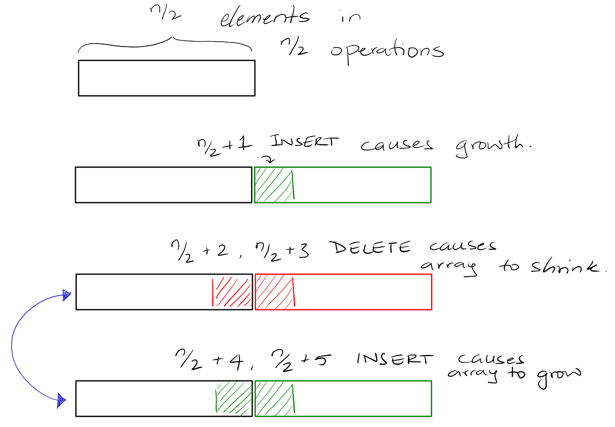
This leads to a situation where the worst case running time is \(\Theta(n^2)\).
This would lead to an amortized time of \(\Theta(n)\)
The problem is that we're too strict about the load-factor. There are not enough
operations for the potential to built up.
Solution: We double when the array size when inserting into a full array. We
halve the array size when a delete would cause the array to be less than quarter
full.
Analysis: Let \(\alpha_i\) be the load factor after the \(i\)th operation.
\[
\Phi(A_i) = \begin{cases}
2n_i - s_i &\text{ if } \alpha_i \geq \frac12 \\
\frac{s_i}{2} - n_i &\text{ if } \alpha_i < \frac12 \\
\end{cases}
\]
Space Overhead
The overhead of a data structure, currently storing \(n\) elements, is the
amount of memory usage beyond the minimal required to store \(n\) elements.
Vector: \(\Theta(n)\), in the worst case, when we are shrinking the array
from \(4n\) to \(2n\) we require a total of \(6n\) space (old and new array
combined). Therefore, the worst-case overhead requirement is \(5n\).
<< Insert diagram for this case >>
Lower bound for array: At some point in time, \(\Omega(\sqrt n)\) overhead
is necessary, for any data structure that supports inserting elements and
locating any element in some order, where \(n\) is the number of elements stored
in the data structure.
Proof: Consider the following sequence of operations for any \(n\).
INSERT(a1)
INSERT(a2)
...
INSERT(an)
After inserting \(a_n\), let \(k(n)\) be the number of memory blocks occupied by
the data structure. Let \(s(n)\) be the size of the largest of these blocks. For
the vector solution, \(k(n) = \Theta(1)\) and \(s(n) = \Theta(n)\). In a linked
list, \(k(n) = \Theta(n)\), \(s(n) = \Theta(1)\).
Since any element can be located, the data structure must store all the
elements in memory. Hence, \(k(n) \cdot s(n) \geq n\). At this time, the
overhead is at least \(k(n)\) to store book-keeping information for each block
(memory address) since you need to keep track of these memory blocks.
Furthermore, immediately after the allocation of the block of size \(s(n)\), the
overhead is at least \(s(n)\) (since it has yet to be populated).
Therefore, the worst-case overhead is at least \(max(k(n), s(n))\).
Since \(s(n) \cdot k(n) \geq n\), at some point, the overhead is at least
\(\sqrt n\) (if not, the product would be less than \(n\)).
Optimal Solution
Let Allocate(s) be a function that returns a new block of size \(s\) and
Deallocate(B) be a function that frees the space used by the given block
\(B\). Let Reallocate(B, s) be a function that if possible, resizes block
\(B\) to size \(s\), otherwise allocate a block of size \(s\), copies the
content of \(B\) into the new block and deallocates \(B\) and returns the new
block. We can assume Allocate and Reallocate are constant time \(O(1)\) and
the Reallocate takes \(O(s)\) time in the worst-case.
NOTE: There are some programming languages that initialize and clear memory
block when they allocate and deallocate. For such languages, the running time
would take \(O(s)\).
Approaches That Do Not Work
Approach 1
Try to store elements in \(\Theta(\sqrt n)\) blocks, and the size of the largest
block is also \(\Theta(\sqrt n)\).
B1: size = 1
B2: size = 2
B3: size = 3
...
Bk: size = k
Every time we insert an element, if there is not space we increase the size of
the block by 1.
The total number of elements in the first \(k\) blocks is going to store
\(k(k+1)/2\). The number of blocks required to store \(n\) elements would be:
\[
\begin{align}
\frac{k(k+1)}{2} &= n \\
k &= \lceil \frac{\sqrt(1 + 8n) - 1}{2} \rceil
\end{align}
\]
This gives us a solution with space \(\Theta(\sqrt n)\).
Issue: The locate(i) function is in block:
\[
\lceil \frac{\sqrt(1 + 8n) - 1}{2} \rceil
\]
However, the square root function is not possible in constant time.
Approach 2
Try to store elements in \(\Theta(\sqrt n)\) blocks, and the size of the largest
block is also \(\Theta(\sqrt n)\).
B1: size = 1
B2: size = 2
B3: size = 4
...
Bk: size = 2^k
Locate(i) to find which block contains \(i\), we can take the number of bits
in the binary expression of \(i+1\) - 1. This can be done in constant on CPUs.
Issues: Size of the largest block is \(\Theta(n)\) (\(2^k\)). Immediately
after allocating the largest block, the overhead space is an order on n.
Solution
Our solution contains two types of blocks, an "index block" and "data blocks".
The index block stores pointers to the data blocks which is stored as a vector.
The data blocks store the actual elements in the array. We have \(d\) data
blocks that are non-empty.
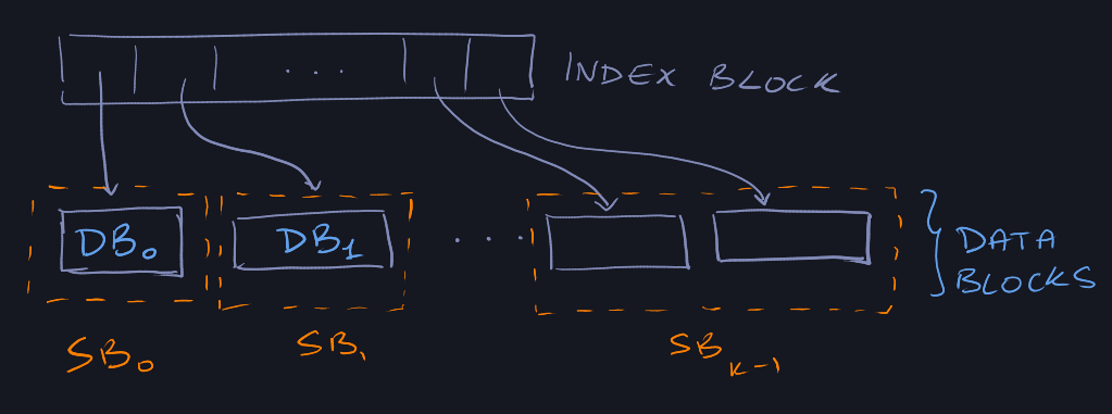
A super block (\(SB_0\), \(SB_1\), ..., \(SB_{s-1}\)) are groups of data blocks.
Data blocks in the same super block are of the same size.
When super block \(SB_k\) is fully allocated, it consists of \(2^{\lfloor k/2
\rfloor}\) data blocks, each of which are \(2^{\lceil k/2 \rceil}\) in size.
Therefore, the size of \(SB_{k}\) has \(2^k\) elements.
Only \(SB_{s-1}\) might not be fully allocated.
Reference: Resizable Arrays in Optimal Time and
Space
Operations
Supporting random access in O(1)
LOCATE(i): Return the address of the \(i\)th element.
Let \(r\) be the binary expression of \((i + 1)\). The super block that contains
this element is element \(e\) of data block \(b\) of super block \(k\), where:
\[
k = |r| - 1
\]
\(b\) is the \(\lfloor k/2 \rfloor\) bits of \(r\) immediately after the leading
1-bit.
\(e\) is the last \(\lceil k/2 \rceil\) bits of \(r\).
Where \(|r|\) is the number of bits in \(r\).
5 = (5+1) = 110 = 1, 1, 0
But to index the element, we need to first calculate how many data blocks are
before the kth super block. This is because we only know the relative index of
the data block within the super block.
\[
\begin{align}
p &= \sum_{j=0}^{k-1} 2^{\lfloor j/2 \rfloor} \\
&= 2 * (2^{k/2} - 1) & \text{if k is even} \\
&= (3 * 2^{(k-1)/2}) - 2 & \text{if k is odd}
\end{align}
\]
Return the location of element \(e\) in data block \(DB_{p+b}\) (we can get this
from the index block in constant time.)
Updates:
Some easy to maintain book-keeping information:
- \(n\) Number of items in the array.
- \(s\) Number of super blocks in the array.
- \(d\) Number of non-empty data blocks.
- \(d_e\) Number of empty data blocks (0 or 1).
- \(d_s\) The size and occupancy of the last non-empty data block.
- \(s_s\) The size and occupancy of the last non-empty super block.
- \(i_s\) The size and occupancy of the last non-empty index block.
- The index block is maintained as a vector.
Insert Operation:
-
If \(SB_{s-1}\) (last super block) is full, \(s = s+1\).
-
If \(DB_{d-1}\) is full and there is no empty data block, \(d = d+1\) and
allocate a new data block as \(DB_{d-1}\).
-
If \(DB_{d-1}\) is full and there is an empty data block, \(d = d+1\) and
\(DB_{d-1}\) is the next empty data block.
-
Store \(x\) in \(DB_{d-1}\).
Delete Operation:
-
Remove the last element.
-
If \(DB_{d-1}\) is empty then \(d = d-1\). If \(d_e = 1\), then we deallocate
the empty data block. If not, set \(d_e = 1\).
-
If \(SB_{s-1}\) is empty, \(s = s - 1\)
Analysis
\(S = \lceil \lg (1+n) \rceil\).
Proof: The number of elements in the first s super blocks:
\[
\sum_{i=0}^{s-1} = 2^s - 1
\]
If we let this equal \(n\), then \(s=\lg(1+n)\). For slightly smaller \(n\), the
same number of super blocks are required, hence we take the ceiling.
The number of data blocks is \(O(\sqrt n)\). Proof: As there is at most one
empty data block, it suffices to prove that \(d = O(\sqrt n)\):
\[
\begin{align}
d &\leq \sum_{i=0}^{s-1} 2^{\lfloor i/2 \rfloor} \\
&\leq \sum_{i=0}^{s-1} 2^{i/2} \\
&= \frac{2^{s/2} - 1}{\sqrt(2) - 1} \\
&= O(\sqrt n)
\end{align}
\]
The last data block has size \(\Theta(\sqrt n)\). Proof: Size of \(DB_{d-1}\)
(the last non-empty data block) is \(2^{\lceil (s-1)/2 \rceil}\) which is equal
to \(\Theta(\sqrt n)\). If there is an empty data block, either it's the same
size or twice the size (next super block) which would also be \(\Theta(\sqrt
n)\).
Therefore, the total overhead of the data structure is \(O(\sqrt n)\).
Update time:
Even if the model requires \(O(n)\) time for allocation and deallocation even
then the amortized time is \(O(1)\).
If allocate or deallocate is called when \(n\) is equal to \(n_0\), then the
next call to allocate or deallocate will occur after \(\Omega \sqrt{n_0}\).
To prove this:
Immediately after allocating or deallocating a data block, there is exactly one
empty data block. We only deallocate a data block after two are empty, so we
must call delete as many times as size of \(DB_{d-1}\) which is \(\Omega
(\sqrt{n_0})\).
As we only allocate a data block when this empty data block is full, this
requires \(\Omega \sqrt{n_0}\) insertions.
Summary
The data structure uses the concept of data blocks and super blocks to
facilitate a low overhead resizeable array.
It achieves an overhead space requirement of \(O(\sqrt{n})\).
It maintains Insert, Delete, and Query operations under \(O(1)\) amortized time.
Van Emde Boas Trees
Problem Statement
Maintain an ordered set of \(n\) elements to support:
- Membership (search)
- Successor / Predecessor of a given element (strict)
- Insert / Delete from set
Example: 2, 7, 11, 20, 25.
- Is 11 in the set? Yes.
- Is 12 in the set? No.
- What's the successor of 11? 20.
- What's the predecessor of 3? 2.
- Insert 21.
- Delete 11.
Well-Known Solutions
Binary Search Trees
The most well known solution to this problem is a balanced search tree.
- \(\Theta(\lg n)\) time.
- \(O(n)\) space.
Lower bound for membership under the binary decision tree model is \(\Omega(\lg
n)\).
A binary decision tree model is a binary tree where each node is labelled
\(x < y\) (a comparison between two specific elements). The program execution
corresponds to a root-to-leaf path. A left contains the result of computation.
Decision trees correspond to algorithms that only use comparisons to gain
knowledge about input.
The binary search algorithm is an algorithm on this binary decision tree model.
Proof of lower bound: Any binary decision tree for membership must have
at least \(n+1\) leaves, one for each element + additional leaf for "not found".
As a binary tree of \(n+1\) leaves, the tree must have height \(\Omega(\lg n)\),
since any program execution corresponds to root-to-leaf path, in the worst-case
the algorithm looks for this leaf. Therefore, the algorithm has a running time
lower bound of \(\Omega(\lg n)\).
Dynamic Perfect Hashing
Perfect hashing would achieve \(O(1)\) worst-case time for membership queries.
The INSERT and DELETE operations are \(O(1)\) expected amortized time.
<< read reference posted online >>
This is based on the RAM model and we use input values as memory addresses, and
this is the reason we achieve the constant-running time.
The "expected time" stands for average time.
Hashing also doesn't support predecessor and successor operations efficiently.
Word RAM Model
This model tries to model a realistic computer. In original RAM model you could
store an infinitely precise number. However, in the Word RAM model there is a
maximum number of bits in a word.
-
Word size \(w \geq \lg n\). Think of it as the minimum size of a pointer. We
need a pointer/memory address to each element.
-
\(O(1)\): "C-style" operations.
-
Universe size: \(u\), where elements have values in \([0, u)\) from
\(\mathbb{Z}\).
-
\(w \geq \lg u\) since we use \(w\) bits to encode any element from universe.
Preliminary Approaches
Direct Addressing
Uses a bit-vector of length \(u\).
Example, let \(u=16\), \(n=4\), \(s\) is the current set containing 1, 9, 10,
15.
\[
B = [0, 1, 0, 0, , ... 1, 0, ..., 1]
\]
\(B[i] = 1\) if \(i\) is in the set \(s\).
- Insert/Delete/Membership: \(O(1)\).
- Successor/Predecessor: \(O(u)\).
- Space: \(O(u)\)
Carved Bit-Vector
Carve the bit-vector into widgets of size \(\sqrt{u}\) (assume \(u=2^{2k}\)).
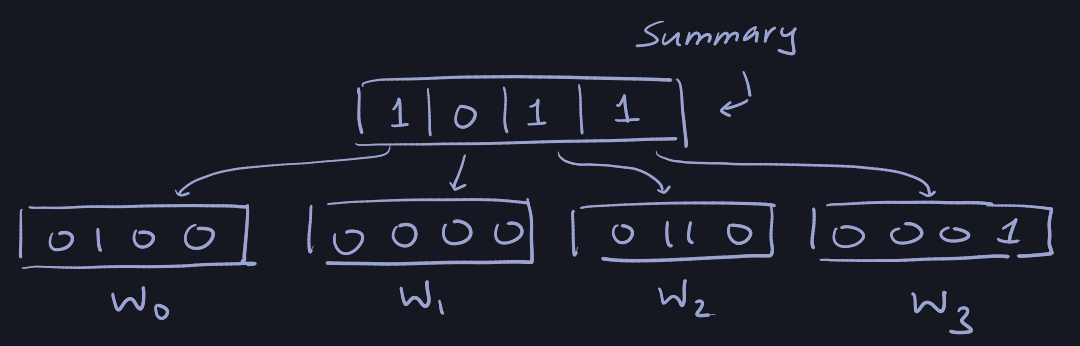
\(W_i[j]\) denotes \(i \sqrt{u} + j\), \(j = 0, \dots \sqrt{u} -1\). The summary
widget has size \(\sqrt{u}\) and summary\([i] = 1\) iff \(W_i\) contains a
\(1\).
Aliases: \(high(x) = h(x)\) and \(low(x) = l(x)\)
- \(h(x) = \lfloor x / \sqrt{u} \rfloor\).
- \(l(x) = x \text{ mod } u\).
- $x = $ \(h(x) \sqrt{u}\) + \(l(x)\).
- When \(x\) is represented as a binary number with \(\lg u\) bits then
\(h(x)\) is simply the highest \((\lg u) / 2\) bits and \(l(x)\) is the
\((\lg u)/2\) bits.
The algorithms then are performed by doing:
-
Membership(x): \(W_{h(x)}[l(x)]\) is checked: \(O(1)\).
-
Successor(x): We search to the right in the widget that \(x\) belongs to. If
no elements are found, then we search the summary block for the next widget
with a value in it. In that widget, we search all the values. This can be done
in \(O(\sqrt{u})\).
-
Predecessor(x): Same as Successor(x) but in the reverse direction. This can be
done in \(O(\sqrt{u})\).
-
Insert(x): We just insert the element in the corresponding widget and update
the summary widget to 1 for the corresponding widget. This can be done in
\(O(1)\).
-
Delete(x): Set the position of \(x\) within it's widget to \(0\) and then
check if the entire widget is empty and update the summary block. This can be
done in \(O(\sqrt{u})\).
The space overhead for this solution is \(O(u)\).
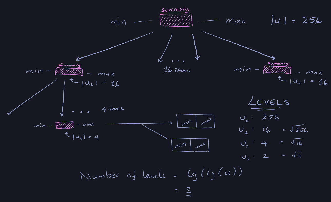
Recursive Splitting Of Universe
The best we can hope for
\[
T(u) = T(\sqrt{u}) + O(1)
\]
Let \(m = \lg u\), so that \(u = 2^m\) then
\[\begin{align}
T(2^m) &= T(2^{m/2}) + O(1) \\
S(m) &= S(m/2) + O(1) \\
S(m) &= O(\lg m) + O(1) \\
T(u) &= O(\lg \lg u)
\end{align}\]
Now we design this recursive approach:
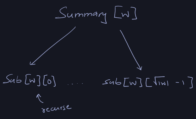
And for implementation purposes, it's easier to understand it as the following
diagram:
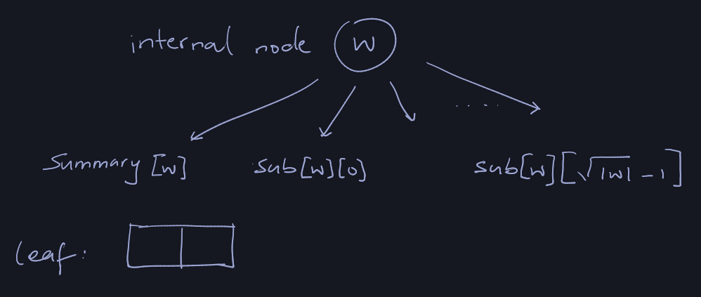
Now we implement the algorithms:
Membership(w, x)
    if |w| = 2
        return w[x]
    else
        return Membership(Sub[w][high(x)], low(x))
\[
T(u) = T(\sqrt{u}) + O(1) = O(\lg \lg u)
\]
Insert(w, x)
    if |w| = 2
        w[x] = 1
    else
        Insert(Sub[w][high(x)], low(x))
        Insert(Summary[x], high(x))
This requires two recursive calls
\[
\begin{align}
T(u) &= 2T(\sqrt{u}) + \Theta(1) \\
m &= \lg u \\
T(2^m) &= 2T(2^{m/2}) + \Theta(1) \\
S(m) &= T(2^m) \\
S(m) &= 2 S(m/2) + \Theta(1) \\
S(m) &= \Theta(m) \\
T(w) = \Theta(\lg u)
\end{align}
\]
Therefore, the running time of the Insert operation is \(\Theta(\lg u)\).
Successor(w, x)
    if (|w| = 2)

    j = Successor(sub[w][high(x)], low(x))
    if j < infinity
        return high(x) * \sqrt(|w|) + j
    else
        i = Successor(summary[w], high(x))
        j = Successor(sub[w][i], -infinity)
        return i * \sqrt(|w|) + j
This requires three recursive calls
\[
\begin{align}
T(u) &= 3T(\sqrt{u}) + \Theta(1) \\
m &= \lg u \\
T(2^m) &= 3T(2^{m/2}) + \Theta(1) \\
S(m) &= T(2^m) \\
S(m) &= 3 S(m/2) + \Theta(1) \\
S(m) &= \Theta(...) \\
T(w) = \Theta((\lg u)^{\lg 3})
\end{align}
\]
Van Emde Boas Tree
Compared to the recursive structure, it has two improvements:
- For each widget
w, we store the minimum an maximum value in the widget. If
the set is empty, the both the min and max is -1. This reduces the
requirement of two extra recursive call.
Successor(w, x)
    if x < min[w]
        return min[w]

    else if x >= max[w]
        return infinity

    // sub widget containing x
    w' = sub[w][high(x)]

    if low(x) < max[w']
        return high(x) * \sqrt{|w|} + Successor(w', low(x))

    else
        i = Successor(summary[w], high(x))
        return i * \sqrt(|w|) + min[sub[w][i]]
We compare low(x) against max[w'] since the sub-widget is a sub-universe. It
only contains elements from the universe \(\sqrt{|w|}\) where \(|w|\) is the
universe size of the current \(w\).
This is also why we add \(high(x) + \sqrt{|w|}\) to the result of the recursive
call - it only returns the value for the sub-universe.
Since there is only one recursive call, the running time of the Successor
operation is \(\lg \lg u\) running time.
Insert(w, x)
    if sub[w][high(x)] is empty:
        Insert(Summary[w], high[x])

    Insert(sub[w][high(x)], low(x))

    if x < min[w] or min[w] = -1
        min[w] = x
    if x > max[w]
        max[w] = x
This running time is \(O(\lg u)\) running time.
To fix this issue, we update our data structure in update 2.
- We do not store
min[w] or max[w] in any sub widget of w, we only store it
once in w.
We only maintain a summary in the summary element for elements that are not min
and max.
The Membership function has some trivial changes, checking the min and max
fields before recursive. Therefore, the running time is still \(O(\lg \lg u)\).
The Successor function also has some trivial changes, with still just one
recursive call leading to a running time of \(O(\lg \lg u)\)
Insert(w, x)
    if min[w] = max[w] = -1
        min[w] = x
        max[w] = x

    else if min[w] = max[w]
        if x < min[w]
            min[w] = x
        else
            max[w] = x

    else
        if x < min[w]
            swap(x, min[w])

        else if x > max[w]
            swap(x, max[w])

        w' = sub[w][high(x)]

        Insert(w', low(x))

        if max[w'] == min[w']
            Insert(summary[w], high(x))
If the second recursive call takes place then the first recursive call has a
running time of \(O(1)\) since the sub widget is empty.
\[
T(u) = T(\sqrt{u}) + O(1)
\]
Therefore, the running of the algorithm is \(O(\lg \lg u)\)
Delete(w, x)
    if min[w] = -1
        return

    if min[w] = max[w]
        if x = min[w]
            min[w] = -1
            max[w] = -1

        return

    if min[summary[w]] = -1
        // there are two elements - one in min and one in max
        if min[w] = x
            min[w] = max[w]
        else if max[w] = x
            max[w] = min[w]
        return

    if min[w] = x
        // the first subwidget that has atleast one element
        j = min[summary[w]]

        min[w] = min[sub[w][j]] + j \sqrt{|w|}
        x = min[w]

    if max[w] = x
        // the last subwidget that has atleast one element
        j = max[summary[w]]

        max[w] = max[sub[w][j]] + j \sqrt{|w|}
        x = max[w]

    // get the subwidget that contains x
    w' = sub[w][high(x)]
    Delete(W', low(x))
    if min[w'] == -1
        Delete(summary[w], high(x))
Again, it looks like there are two recursive calls but for min[w'] = -1 to be
true, the first recursive call would only take constant time. Therefore, the
number of recursive calls in total is one.
Therefore, the running time of this algorithm is \(O(\lg \lg u)\).
Space Cost Analysis
Let \(S(u)\) be the space of the data structure. The space taken by the pointers
and the min/max field are going to be \(\Theta(\sqrt{u})\).
\[
S(u) = (\sqrt{u} + 1) S(\sqrt{u}) + \Theta(\sqrt{u})
\]
This is going to be space of \(O(u)\).
Sqrt u details
If \(\sqrt{u}\) is not an integer, then we can just take the ceiling of
\(\sqrt{u}\).
\[
T(u) = T(\lceil \sqrt{u} \rceil) + O(1) \leq T(u^{2/3}) + O(1)
\]
Which simplifies to \(O(\lg \lg u)\).
Summary
van Emde Boas Trees is a recursive structure where we store a min and max for
each widget and a summary for all the other elements in the widgets.
For an element x, high(x) (the first half of the bits in the binary
representation) identifies the sub-widget that contains element x. low(x)
(the lower half of the bits) is the value of x within the sub-widget
(sub-universe).
- Space overhead: \(O(u)\)
- Membership: \(O(\lg \lg u)\)
- Successor and Predecessor: \(O(\lg \lg u)\)
- Insert and Delete: \(O(\lg \lg u)\).
Fast Tries
The objective of the data structure is the same as van Emde Boas Trees but we
wish to reduce the space complexity of the data structure to \(O(n)\) rather than
\(O(u)\) for cases where the universe size is really large.
Preliminary Approach
Let the following be the case: u=16, n=4, S={1,9,10,15}.
Binary Tree Approach
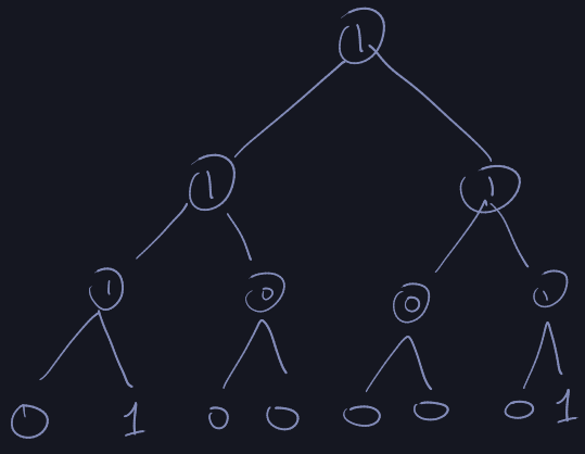
We store elements as a doubly-linked list.
We store 3 different data structures: bit-vector, tree, and a doubly-linked
list.
- Membership: \(O(1)\)
- Successor(x):
- if \(x \in S\) then we use the doubly-linked list - \(O(1)\).
- else We walk up the tree till we find the
1 node. This node must have a
one child. Then there are two cases:
- if it's a right child, we need the smallest element \(O(\lg u)\).
- if it's a left child, we need the largest element \(O(\lg u)\) would be
the predecessor, then we use the linked list to find the successor.
- Insert/Delete: \(O(\lg u)\)
The bit vector requires \(O(u)\) space.
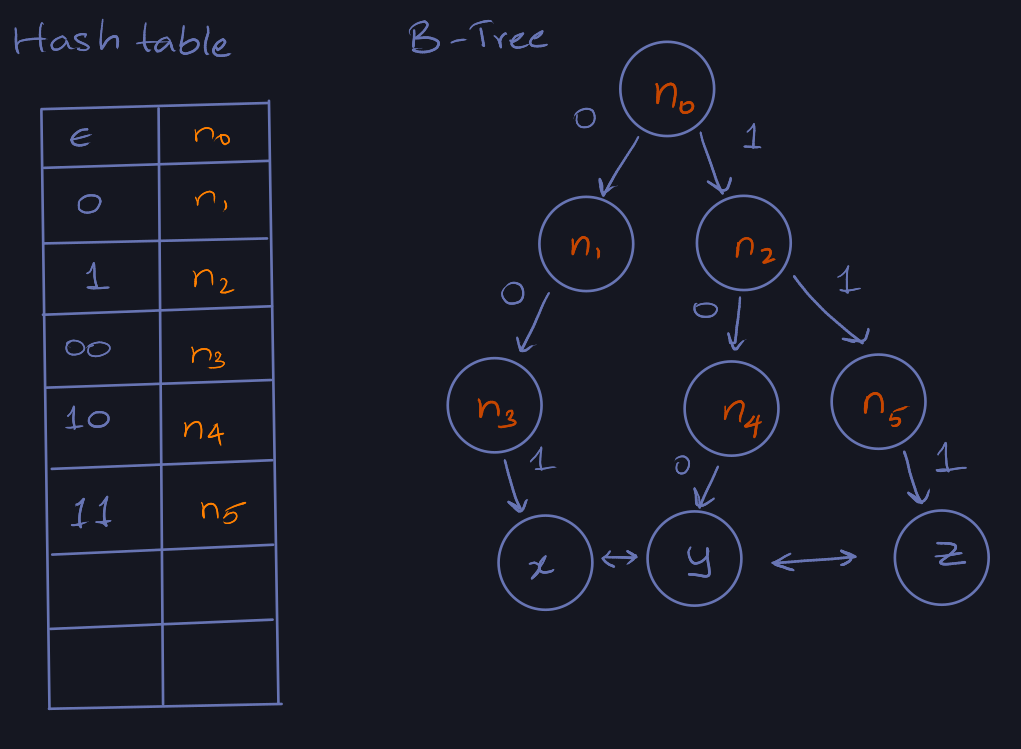
X-fast Tries
From this we learn that we can't keep the bit-vector. We keep the doubly-linked
list. And we only keep only the 1 nodes from the tree.
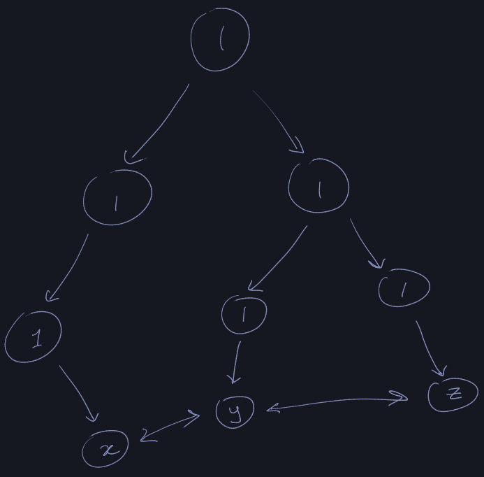
Successor
How to locate the lowest 1 node from the leaf x to the root?
Solution: Each ancestor of x corresponds to a prefix of the binary expression
of x. Consider x=13 which is x=1101 if we see a 1 we go to the right
child and if we see a 0 then we go to the left child.
Using such a prefix, as a key for any 1-node. We store it in a dynamic perfect
hashing table. A dynamic hashing table of \(m\) keys, \(O(m)\) space and \(O(1)\)
worst-case membership and \(O(1)\) amortized insert and delete.
The lowest 1 node that is an ancestor of x corresponds to the longest
prefix of x that is in the hash table. To find this longest prefix, we can
perform a binary-search over the length of the prefix. Therefore, we can find
the lowest 1 node in \(O(\lg \lg u)\) time.
For each entry added to the data structure, we need to store at most \(\lg u\)
nodes in the hash table. Since the total number of nodes is \(n\), the worst-case
over head space in the hash table would be \(O(n \lg u)\).
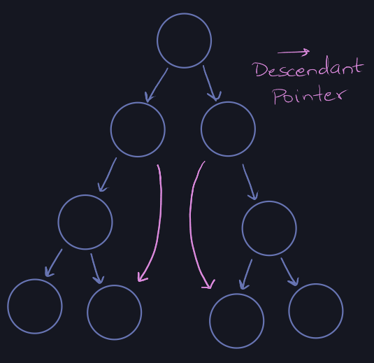
If we follow the tree to find the successor or predecessor it would take \(O(\lg
u)\) time. Therefore, we store a descendant pointer to the smallest leaf.
-
If the node has a 1-child as its right child, we store a descendant pointer to
the smallest left of the right sub-tree (successor).
-
If the node has a 1-child as its left child, we store a descendant pointer to
the largest leaf of its left sub-tree (predecessor).
If this node has a 1 child as it's right child, we follow the descendant
pointer to find the successor.
If this node has a 1 child as it's left child, we follow the descendant
pointer to find the predecessor and then use the doubly-linked list to find the
successor.
Note: Only nodes with exactly one child require descendant pointers since if a
node has two children, then a higher prefix would have matched to a lower node.
We are finding the closest 1-node to the queried x, which much have one child
or be the element itself.
Other Operations
Space Analysis
- List: \(O(n)\)
- Hash table: \(O(n \lg u)\)
- Tree: \(O(n \lg u)\)
Therefore, the total space is \(O(n \lg u)\).
Summary
The x-fast trie tries to not use \(O(u)\) space by maintaining three data
structures: A doubly-linked list, a binary tree, a hash-table. It uses the
hash-table and the double linked list for successor and predecessor operations.
It maintains additional descendant points to optimize locating the successor and
predecessor.
- Space: \(O(n \lg u)\) (for tree and hash-table)
- Successor and Predecessor: \(O(\lg \lg u)\)
- Member: \(O(1)\)
- Insert and Delete: \(O(\lg u)\) amortized expected.
Y-fast Tries
Indirection: We cluster elements of \(S\) into consecutive groups of size \((\lg
u)/4\) to \(2\lg u\). From this we get that the number of groups is \(O(n / \lg u)\).
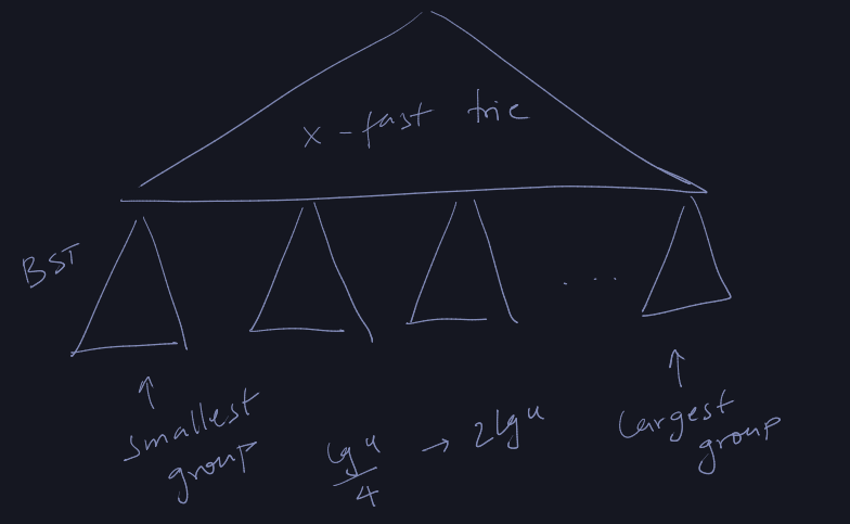
We then store elements of each group in a balanced binary search tree. We
maintain a set of representative elements, one per group, stored in a x-fast
tries structure.
A group's representative does not have to be in \(S\), but it has to be strictly
between the max and the min elements of the preceding and succeeding groups
respectively.
If we have a set number of elements then we just set each group size to be \(\lg
u\) size and then pick any element in the group to be the representative.
Space Analysis
X-fast tries uses:
$$
O(\frac{n}{\lg u} \lg u) = O(n)
$$
BST: \(O(n)\)
Operations Analysis
Membership:
If \(x\) is stored in the x-fast trie then check the corresponding BST to see if
\(x \in S\) and if \(x\) is not present, then we find the predecessor and the
successor in the x-fast trie. \(x\) must be present in one of these BSTs if it is
present.
It takes \(O(1)\) to check if \(x\) in x-fast trie and the binary search tree search
takes \(\lg \lg u\) time.
Running time: \(O(\lg \lg u)\)
Predecessor/Successor:
This has a similar idea to membership and has a running time of \(O(\lg \lg u)\).
Insert/Delete:
We use x-fast trie to locate the group that \(x\) is in. Then we just insert \(x\)
into the balanced binary search tree of that group or we just delete \(x\) from
the binary search tree of that group.
We need to ensure the group size must remain between \(1/4 \lg u\) and \(2 \lg u\).
To achieve this, when a group is of size greater than \(2 \lg u\) (after insert),
we just split the group into two groups of about \(\lg u\) size each. When the
group size is less than \(1/4 \lg u\) (after delete) we merge it with an adjacent
group. If this causes a group to be too large, we can split again.
- Find element position: \(O(\lg \lg u)\)
- Insert into BST: \(O(\lg \lg u)\)
- Maintain the group size: \(O(\lg u)\) and \(O(1)\) amortized.
The split and merge operations can be done using in-order traversal and can be
done linearly to the tree size (\(O(\lg u)\)). Then we need to insert something
into the x-fast trie which is \(O(\lg u)\) amortized expected time.
This only merge and split only takes place every \(\Omega(\lg u)\) insert delete
operations. This is \(O(1)\) amortized expected running time for this merge and
split operations.
Therefore the total worst-case amortized expected running time is \(O(\lg \lg
u)\).
Indirection is a general approach to decreasing space cost.
Summary
To avoid using the \(O(n \lg u)\) space of the x-fast trie, we only store \(\lg u\)
items in the x-fast trie. We maintain BST groups which have representatives
stored in the x-fast trie. The groups are sized dynamically between \(1/4 \lg u\)
and \(2 \lg u\).
- Space: \(O(n)\)
- Membership: \(O(\lg \lg u)\)
- Predecessor and Successor: \(O(\lg \lg u)\)
- Insert and Delete: \(O(\lg \lg u)\) amortized expected.
The insert and delete require \(O(\lg u)\) time in the worst-case to maintain
group size. However, this is amortized to \(O(1)\) over \(n\) operations.
Self-adjusting Lists
Problem Statement
Linear search! We have a list of \(n\) elements and we are required to perform a
linear search over these elements for a particular element \(x\). The worst-case
running time for this is \(n\) comparisons.
If all elements have equal probability of search then the expected time is
\(\frac{(n+1)}{2}\) if it is present in the list and \(n\) for unsuccessful
search.
\[
\begin{align}
\text{Cost } &= \sum_{i=1}^{n} \frac{1}{n} i \\
&= \frac{n + 1}{2}
\end{align}
\]
-
What if probabilities of access differ between elements? Let \(p_i\) be the
probability of element \(i\) being requested.
-
What if the independent probabilities are not given?
-
How do these solutions compare with the best we could do?
Independent And Equal Probabilities
If probabilities are the same and independent it doesn't matter how you change
the structure.
The best you can hope for is \(\frac{n+1}{2}\) number of comparisons.
Fixed Probabilities And Lists
The probabilities and the list is fixed so that it cannot be changed. In this
case, we want to minimize the expected number of comparisons.
\[
\sum_{i=1}^{n} i p_i
\]
To solve this, we can use a greedy algorithm and pick the element with the
highest probability to be first and so on.
This is the static optimal solution \(S_opt\).
There are cases where binary search does not perform as well as an optimized
linear search. Binary search has a low cache-hit rate which may cause slowdowns
in the real world.
Changing Unknown Probabilities
How do we adapt to changes in probabilities or "self-adjust" to do better?
We should move elements forward as accessed. There are many heuristics on how to
move elements forward:
- Move-to-front (MTF): After accessing an item, we move that item to the front
of the list.
- Transpose (TR): After accessing an item exchange it with an immediate
preceding item.
- Frequency Count (FC): We maintain a frequency count for each item, initially
- Increase the counter by 1 whenever it is accessed. Maintain the list so
that items are in decreasing order of frequency count.
In practice, usually they use MTF.
Static Optimality Of Move-to-front
Compare cost of MTF with the cost of \(S_opt\) (static optimal) solution.
For the model, we start with an empty list. We scan for elements requested,
if it's not present in the list we Insert (and charge as if found at end of
list) then apply heuristic to self-adjust.
The cost is the number of comparisons performed over a sequence of operations.
Consider an arbitrary list, but focus on search for \(b\) and \(c\), and in
particular, we focus on "unsuccessful" comparisons where we compare query value
\(b\) or \(c\) against \(c\) or \(b\) respectively.
Assume request sequence has \(k\) \(b\)'s and \(m\) \(c\)'s, without loss of generality,
we assume \(k \leq m\).
\(S_{opt}\) order is [c, b] because \(c\) is accessed more times than \(b\). There are
\(k\) unsuccessful comparisons since we only miss the \(b\)s.
For the worst-case for the MTF algorithm, we alternate between \(b\) and \(c\)s,
therefore the pattern looks like \(c^{m-k} (bc)^k\). From this, we get that the
maximum number of comparisons is \(2k\).
This holds for any list for any pair of elements. Therefore, if we sum over all
pairs of elements, we find the total number of unsuccessful comparisons of MTF
is less that equal to 2 times total number of unsuccessful comparisons of
\(S_{opt}\).
The number of successful comparisons of MTF and \(S_{opt}\) are equal, the order
doesn't matter for the successful comparisons.
Therefore, cost of \(MTF \leq 2 S_{opt}\).
This bound is tight. Given \(a_1\), \(a_2\), \(\dots\), \(a_n\), we repeatedly ask for
the last element in the list. The cost of MTF would be \(n\) for each search. For
the \(S_{opt}\), the cost would be \((n+1) / 2\).
From some sequences, MTF does a lot better than \(S_{opt}\). Consider the request
sequence: \(a_1^n\), \(a_2^n\), \(\dots\), \(a_n^n\). For such a sequence, we have the
following costs:
\[
\begin{gather}
\frac{[1 + (n-1)] + [2 + (n-1)] + \dots + [n + (n-1)]}{n^2} \\
= \frac{3}{2} - \Theta(\frac{1}{n})
\end{gather}
\]
Therefore, we find that MTF performs the search in constant amortized time.
Dynamic Optimality Of Move-to-front
Online Vs Offline Algorithms
-
Online: Must respond as requests comes, without knowledge of the future.
-
Offline: The algorithm gets to see the entire schedule and determine how
to proceed.
Competitive Ratio of an algorithm is the worst-case of the online time of
using the algorithm divided by the optimal offline time.
\[
\text{Competitive Ratio } = \frac{\text{Online time of Alg.}}{\text{Optimal Offline time}}
\]
A method if competitive if this ratio is a constant.
For the cost model there are two parts:
-
Search for or change element at position \(i\): we scan to location \(i\) at cost
\(i\).
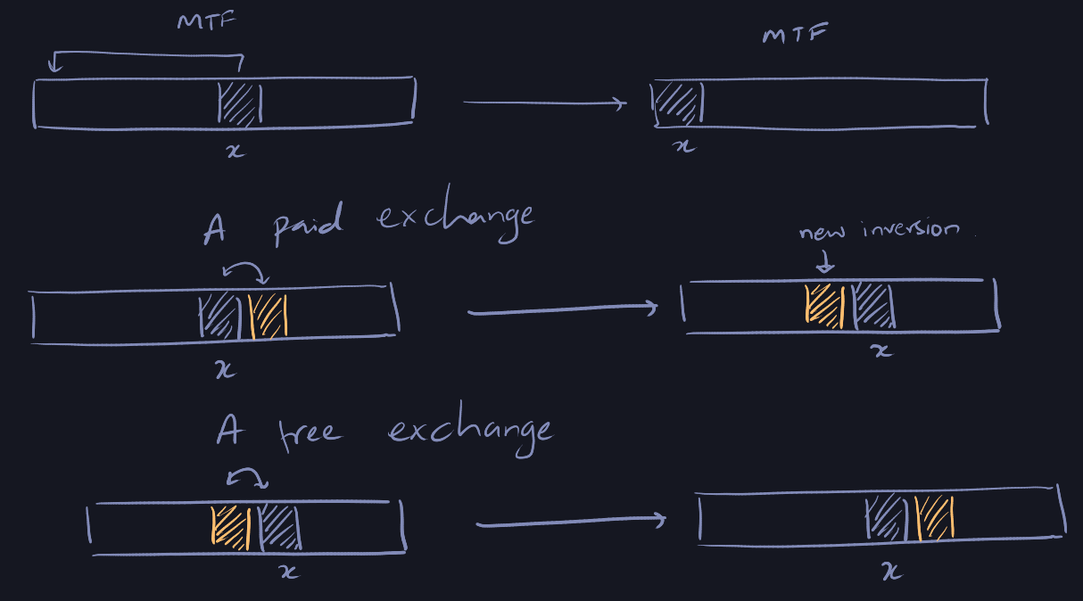
-
Free exchanges: exchanges (swaps) between adjacent elements required to move
element \(i\) closer to the front of the list.
-
Paid exchanges: Any other exchanges (swapping), moving element further from
the front, costs 1.
It's okay to consider moving elements closer to the front "free" since we have
to anyway perform a linear search to the element. Therefore, the number of swaps
is going to be a constant multiple of the number of comparisons to find the
element. This does not change the cost asymptotically, just by a constant factor.
- Access: costs \(i\) if element is in position \(i\).
- Delete: costs \(i\) if element is in position \(i\).
- Insert: costs \(n+1\) if \(n\) elements are already there.
The above costs are the costs before self-adjusting.
The request sequence \(S\) has a total of \(M\) queries and a maximum \(n\) data
values. We start with an empty list.
The cost for a search that ends by finding the element in position \(i\) is \(i\)
plus the number of paid exchanges.
-
Let \(C_A(S)\) be the total cost of all the operations for algorithm \(A\), not
counting paid exchanges.
-
Let \(X_A(S)\) be the number of paid exchanges.
-
Let \(F_A(S)\) be the number of free exchanges.
\[
X_{MTF}(S) = X_{TR}(S) = X_{FC}(S) = 0
\]
This is because in all the above algorithms (MTF, TR, FC) we only move elements
to the front.
For any algorithm \(A\), \(F_A(S) \leq C_A(S) - M\). After accessing the \(i\)th
element, there are at most \(i-1\) free exchanges that can be made.
However, to perform competitive analysis we need to know the optimal offline
algorithm. For the question of self-adjusting lists, this is not a known
solution. Therefore, we compare it against a general case (any algorithm).
\[
C_{MTF}(S) \leq 2 C_A(S) + X_A(S) - F_A(S) - M
\]
We try to prove the above for any algorithm \(A\) starting with the empty list.
We run algorithm \(A\) an \(MTF\), in parallel, on the same request sequence \(S\).
Then the potential function \(\Phi\) is defined as the number of inversions
between MTF's list and A's list.
An inversions is when a pair of elements, say \(i\) and \(j\), appear in different
orders in the two lists. That is, either \(i\) before \(j\) or \(j\) before \(i\). We
consider all pairs to find the total number of inversions.
Since we start with an empty list, the initial potential is \(0\) and \(\Phi \geq
0\) since the number of inversions cannot be negative.
Now we bound the amortized time of access for a particular element.
Consider access by \(A\) to position \(i\) and access by \(MTF\) to position \(k\). Let
the element being accessed by \(x\).
Let \(X_i\) be the number items preceding the searched element in MTF's list, but
not in A's list. So, the number items preceding the searched element in both
lists is \(k - 1 - X_i\).
Moving \(x\) to front in MTF's list creates \(k- 1- X_i\) inversions. It would
destroy \(X_i\) other inversions (items before in MTF's list).
So the amortized time is \(k\) + \((k - 1 - X_i)\) - \(X_i\) = \(2(k-X_i) -1\).
Since \(k-1-X_i \leq i - 1\) (elements preceding in both lists is less that in
one), \(k-X_i \leq i\) holds.
Therefore, amortized time of access is at most \(2i - 1 = 2C_A - 1\), where \(C_A\)
is the cost of access for \(A\). The same arguments hold for INSERT and DELETE
operations.
However, this assumes that \(A\) doesn't self-adjust. But \(A\) is also allowed to
self-adjust and this needs to be accounted for in the potential function.
An exchange by \(A\) has zero cost to \(MTF\). So amortized time of an exchange by
\(A\) is just the increase in the number of inversions caused by the exchanges
made by \(A\), that is, \(1\) for any paid exchange made by \(A\), \(-1\) for any free
exchanges.
Therefore, the amortized cost of the general algorithm is:
\[
2 C_A(S) + X_A(S) - F_A(S) - M
\]
MTS is 2-competitive (the competitive ratio is 2):
\[
\begin{align}
T_A(S) &= C_A(S) + X_A(S) \\
X_{MTF}(S) &= 0 \\
T_{MTF}(S) &= C_{MTF}(S) \\
&\leq 2C_A(S) + X_A(S) - F_A(S) - M \\
&\leq 2C_A(S) + X_A(S) \\
&\leq 2C_A(S) + 2X_A(S) \\
&= 2 T_A(S)
\end{align}
\]
This shows that the MTF algorithm at most performs twice as worse as the best
case offline (all information available) algorithm.
Self-Adjusting Binary Search Trees
Problem statement: We're given a sequence of access queries, what is the best
way to organize the values of a search tree?
Model: Searches must start at the root and the cost is the number of nodes
inspected.
Worst-case behaviour: \(\Theta(\lg n)\)
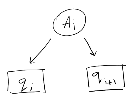
Static Optimal Solution
Given that the probability of access for an element \(A_i\) is \(p_i\). \(q_i\) is the
probability of access for values between \(A_i\) and \(A_{i+1}\) (to fall in the
gap) (\(i = 0, 1, 2, \dots\)).
Let \(A_0 = -\infty\) and \(A_{n+1} = + \infty\) and \(p_0 = 0\) and \(p_{n+1} = 0\).
Let \(T[i, j]\) be the root of the optimal tree on range \(q_{i-1}\) to \(q_j\).
Let \(C[i, j]\) be the cost of the optimal tree rooted at \(T[i, j]\); this is the
sum of the probability of looking for one of the values (or one of the gaps) in
this range times the cost of that item (or gap).
We use a dynamic programming approach to solve this problem:
Observation: First we define \(W[tree]\) (the weight of the tree) as the
probability of being in the tree. The cost of the optimal tree rooted at \(r\):
\[
C[\text{tree rooted at }r] = W[tree] + C[L] + C[R]
\]
We define a table, \(W[i, j]\) to be the probability of accessing any node or gap
in the range \(q_{i-1}, \dots, q_j\) and \(p_i, \dots, p_j\).
\[
W[i,j] = \sum_{k=1}^{j} p_k + \sum_{k=i-1}^{j} q_k
\]
This can be calculated in \(O(n^2)\) time.
\[
W[i, j+1] = W[i,j] + p_{j+1} + q_{j+1}
\]
Dynamic Programming
\[
C[i,j] = \begin{cases}
min_{r=i}^{j}(W[i,j], C[i, r-1], C[r+1, j]) & \text{if } i \leq j \\
0 & \text{if } j = i - 1 \text{ there is one gap}
\end{cases}
\]
OPTIMAL_BST(p, q, n)
  for i = 1 to n + 1
    C[i, i-1] = 0
    W[i, i-1] = q[i-1]

  // l = j - i + 1
  for l = 1 to n
    for i = 1 to n-l+1
      j = i+l-1

      C[i, j] = infinity
      W[i, j] = W[i, j-1] + p[j] + q[j]

      for r = i to j
        t = W[i, j] + C[i, r-1] + C[r+1, j]
        if t < C[i, j]:
          C[i, j] = t
          T[i, j] = r
At the end C[1, n] is the cost of the optimal binary search tree and the root
is stored in T[1, n]. The running time for this algorithm is \(O(n^3)\).
Can build tree using T table.
It is possible to do this in \(O(n^2)\) running time.
Splay Trees
Performing rotations to move a node to the root is a bad approach. This is
because we optimize for the root but every other node in the single rotation was
affected in a bad way.
On accessing a node, we move it (splay it) to the root by a sequence of local
moves, where each move is called a splay step.
Let \(x\) be the node being splayed. \(y\) is the parent of \(x\) and \(z\) is the
parent of \(y\).
There are 3 unique cases:
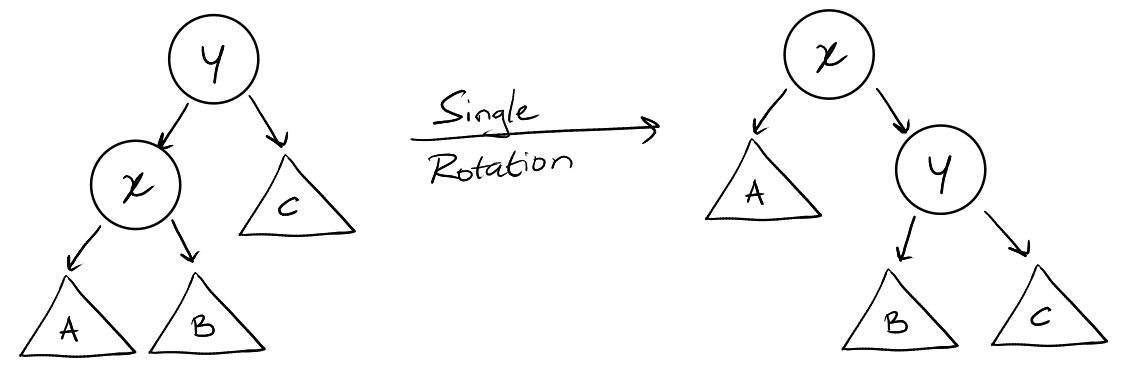
- Zig step: If \(y\) is the root, we rotate \(x\) so that it becomes the root
(single rotation).
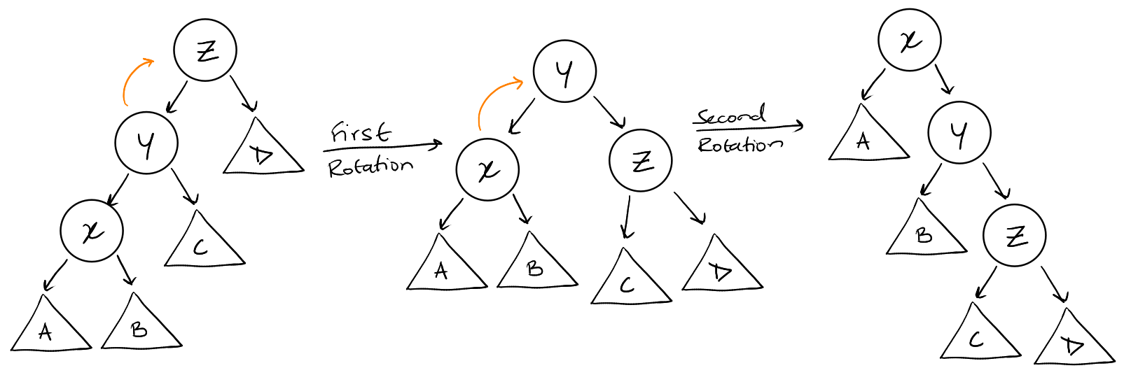
- Zig-Zig step: If \(y\) is not the root and \(x\) and \(y\) are both left or both
right children. We rotate \(y\) and then rotate \(x\).
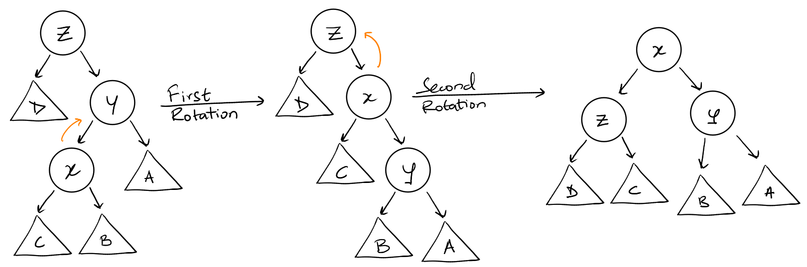
- Zig-Zag step: If \(y\) is not the root and either \(y\) is the left child and \(x\)
is the right child or vice-versa. We perform a double rotation on \(x\).
The cost of splaying a node \(x\) at depth \(d\) is \(O(d)\).
Splaying roughly halves the length of the access path.
Definitions:
- \(w(i)\) is the weight of \(i\) item (always positive weights).
- \(s(x)\) is the size of node \(x\) in the tree, the sum of the individual weights
of all items in the subtree rooted at \(x\).
- \(r(x)\) the rank of the node \(x\), which is \(\lg(s(x))\).
The potential function \(\Phi\) is the sum of the ranks the sum of the ranks of
all its nodes.
\[
\Phi(T) = \sum_{\forall x \ in T} r(x)
\]
Note \(\Phi_i\) is not necessarily non-negative.
\[
\sum_{i=1}^{m} C_i = \sum_{i=1}^{m} a_i + \Phi_0 - \Phi_m
\]
Now the equation still holds but we can't just throw away the potential, we need
to consider it in our upper bound (since it may be negative).
Access lemma: The amortized time to splay a tree with root \(t\) at node \(x\)
is at most:
\[
3(r(t) - r(x)) + 1 = O\left(\lg \frac{s(t)}{s(x)}\right)
\]
Proof: Access Lemma Proof
Note that \(r\left(t\right) = r_k\left(x\right)\) since \(x\) is the root after the splay step.
Balance Theorem: Given a sequence of \(m\) accesses into an n-node splay tree
it has total access time of \(O\left(\left(m+n\right) \lg n + m\right)\).
Proof: We first assign a weight of \(1/n\) to each item. Then, \(1/n \leq s\left(x\right)
\leq 1\). Therefore, the amortized cost of any access is \(3 \lg\left(1\right) - 3 \lg\left(1/n\right) +
1\) which is upper bounded by \(3 \lg n + 1\).
The maximum potential of \(T\) is given by:
\[
\Phi = \sum_{\forall x} r\left(x\right) = \sum_{i=1}^n \lg \left(s\left(i\right)\right) \leq \sum_{i=1}^n \lg 1 = 0
\]
The minimum potential of \(T\) is given by:
\[
\Phi = \sum_{\forall x} r\left(x\right) = \sum_{i=1}^n \lg \left(s\left(i\right)\right) \geq \sum_{i=1}^n \lg \left(1/n\right) = -n \lg n
\]
Therefore, \(\Phi_0 - \Phi_m \leq 0 - \left(-n \lg n\right) = n \lg n\) is the maximum
difference in potential. We substitute this into the amortized cost calculation
to get an upper bound on the amortized cost.
\[
\begin{align}
\text{Total cost } &\leq m \left(3\lg n + 1\right) + \left(n \lg n\right) \\
&\leq m \left(3 \lg n + 1\right) + n \lg n \\
&= O\left(\left(m+n\right) \lg n + m\right)
\end{align}
\]
The worst case can be pretty bad since the splay tree doesn't guarantee any
shape. Therefore, the worst case can be linear time \(O\left(n\right)\). However, if we
access \(m \geq n\) times the amortized cost per access is \(O\left(\lg n\right)\).
Static Optimality Theorem: Given a sequence of \(m\) access into an \(n\)-node
splay tree \(T\), where each item is accessed at least once, then the total access
time is given by:
\[
O\left(m + \sum_{i=1}^n q\left(i\right) \lg \left(\frac{m}{q\left(i\right)}\right)\right)
\]
Where \(q\left(i\right)\) is the access frequency of item \(i\).
Proof: Assign a weight of \(q\left(i\right)/m\) to each item \(i\). Then:
\[
\frac{q\left(x\right)}{m} \leq s\left(x\right) \leq 1
\]
The amortized cost of each access is at most:
\[
\begin{align}
&3 \left(\lg 1 - \lg \left(\frac{q\left(x\right)}{m}\right)\right) + 1 \\
=& 3 \lg \left(\frac{m}{q\left(x\right)}\right) + 1
\end{align}
\]
The maximum potential of \(T\) is given by:
\[
\Phi = \sum_{\forall x} r\left(x\right) = \sum_{i=1}^n \lg \left(s\left(i\right)\right) \leq \sum_{i=1}^n \lg 1 = 0
\]
The minimum potential of \(T\) is given by:
\[
\Phi = \sum_{\forall x} r\left(x\right) = \sum_{i=1}^n \lg \left(s\left(i\right)\right) \geq \sum_{i=1}^n \lg \left(\frac{q\left(i\right)}{m}\right)
\]
Therefore, the difference in potential can be at most:
\[
\sum_{i=1}^n q\left(i\right) \left(3 \lg \left(\frac{m}{q\left(i\right)}\right) + 1\right)
\]
Note that the sum of all \(q\left(i\right)\) is equal to \(m\) which is the total number of
accesses.
\[
\begin{align}
&3 \sum_{i=1}^{n} \left(q\left(i\right) \cdot \lg \left(\frac{m}{q\left(i\right)}\right)\right) + m + \sum_{i=1}^{n} \lg
\frac{m}{q\left(i\right)} \\
&= O\left(m + \sum_{i=1}^{n} q\left(i\right) \lg \left(\frac{m}{q\left(i\right)}\right)\right)
\end{align}
\]
The entropy of the access is given by the following equation:
\[
H = \sum_{i=1}^n q\left(i\right) \lg \left(\frac{m}{q\left(i\right)}\right)
\]
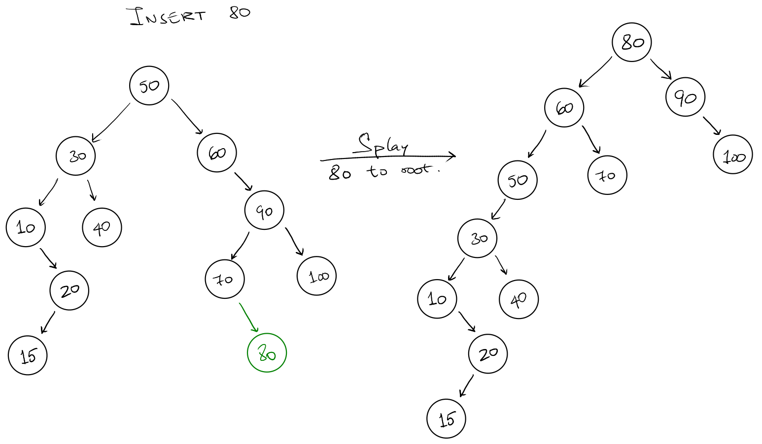
Insert Operation
We insert the value as a new leaf treating the tree as a regular binary search
tree. Then we splay the newly inserted node to the top of the tree.
- Insert the node normally.
- Splay at the new inserted node.
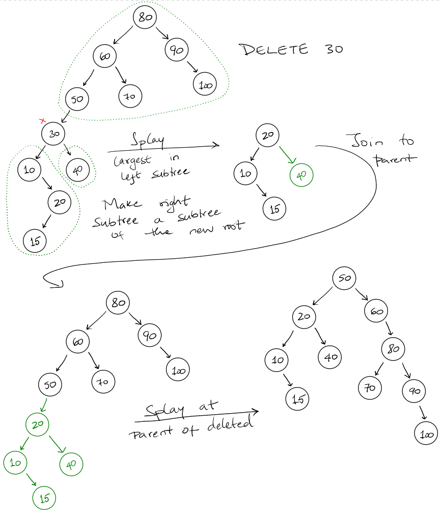
Delete Operation
We first perform a binary search to find the node and then delete it. After we
delete the node, it can have up to 3 separate disconnected trees. The parent,
the left child and the right child.
To combine these 3 trees into one, we splay the largest value in the left
sub-tree. This new root isn't going to have a right child since it's the largest
node. We attach the right sub-tree to the right child of this new root. Then we
attach this tree to the parent. We then splay the tree at the parent of the
delete node.
- Delete node
- Splay largest node in left sub-tree
- Attach right sub-tree to left-subtree
- Attach parent to new tree
- Splay parent of delete node to top.
Summary
-
It's unknown if splay trees are competitive.
-
The average running time of access: \(O(\lg n)\) if number of accesses is
greater than the number of elements.
-
Access lemma: amortized cost is less than \(3(r(t) - r(x)) + 1\).
Entropy
For a set of objects \(S = \{k_1, k_2, \dots, k_n\}\) and a set of probabilities for
each of those objects \(D = \{p_1, p_2, \dots, p_n\}\) and \(p_i\) is the
probability associated with object \(k_i\).
The entropy of \(D\) is given by:
\[
H(D) = -\sum_{i=1}^{n} p_i \lg \left(\pi\right) = \sum_{i=1}^{n} p_i \lg \left(\frac{1}{p_i}\right)
\]
Shannon's Theorem
Consider a sender (Alice) and a receiver (Bob). The sender wants to send a
sequence \(S_1, S_2, \dots, S_m\) where each \(S_j\) is chosen randomly and
independently according to \(D\) (the distribution). So that \(S_j = k_i\) with
probability \(p_i\).
For any protocol the sender and receiver might use, the expected number of bits
required to transmit the sequence using that protocol is at least \(m * H(D)\),
where \(m\) is the length of the sequence and \(H(D)\) is the entropy of the
distribution.
For a uniform distribution, \(p_i = 1/n\) and therefore, \(H(D) = \lg n\). This is
the worst case with maximum entropy.
For a geometric distribution with \(p_i = 1/2^i\) for all \(1 \leq i < m\), the
entropy works out to be:
\[
H(D) = \left[ \sum_{i=1}^{n} \frac{i}{2^i} \right] + \frac{n-1}{2^{n-1}} \leq 2
\]
Therefore, the number of bits required to transmit data is \(2m\) regardless of
the size of \(n\). Note that \(n\) is the number of symbols in the distribution.
Theorem: For any comparison based data structure, storing \(k_1, \dots k_n\)
each associated with probability of \(p_1, \dots p_n\) (to search) the expected
number of comparisons while search for an item is \(\Omega(H(D))\).
Proof: The sender and receiver both store \(k_1, \dots, k_n\) in some
comparison based data structure beforehand. When the sender wants to transmit
\(S\), they perform a search for \(S\) in the data structure. The result of the
comparisons form a sequence of 1s to encode true and 0s for false. This is sent
to the receiver.
On the receiving end, the receiver runs the search algorithm without knowing the
value of \(S\). This can be done since the receiver is doing exactly the same
comparisons and knows the result of the comparison. This way the sender can
transmit \(S\) to the receiver.
By applying Shannon's Theorem, the expected number of bits required to transmit
\(S_1, \dots, S_m\) using this approach is at least \(m \cdot H(D)\). However, the
expected number of bits to transmit the sequence must be less than or equal to
the number of comparisons to search in the data structure.
Therefore, the number of comparisons required is at least \(m \cdot H(D)\).
Static Optimal Binary Search Tree
We start with the assumption that all elements in the request sequence are in
the tree. Let \(p_i\) be the probability of access of \(A_i\) and in this case, the
entropy would be:
\[
H(D) = - \sum_{i=1}^{n} p_i \lg p_i
\]
The expected cost of the static optimal binary search tree would be greater than
or equal to the entropy (\(H\)).
If not all request elements are in the tree, let \(q_i\) be the probability of
accessing a gap \((A_i, A_{i+1})\). For this the entropy of the access would be:
\[
H(D) = - \sum_{i=1}^{n} p_i \lg p_i - \sum_{i=1}^{n} q_i \lg q_i
\]
However, constructing optimal binary search trees are expensive (\(O(n^2)\)),
therefore we consider a NEARLY optimal binary search tree.
We first convert the gaps into items in the tree with dummy nodes.
Goal: Build a BST such that the expected query time if \(O(H+1)\). We say
\(O(H+1)\) since sometimes \(H \propto 1/n\) and therefore \(H+1\) ensures that it is
at minimum constant time.
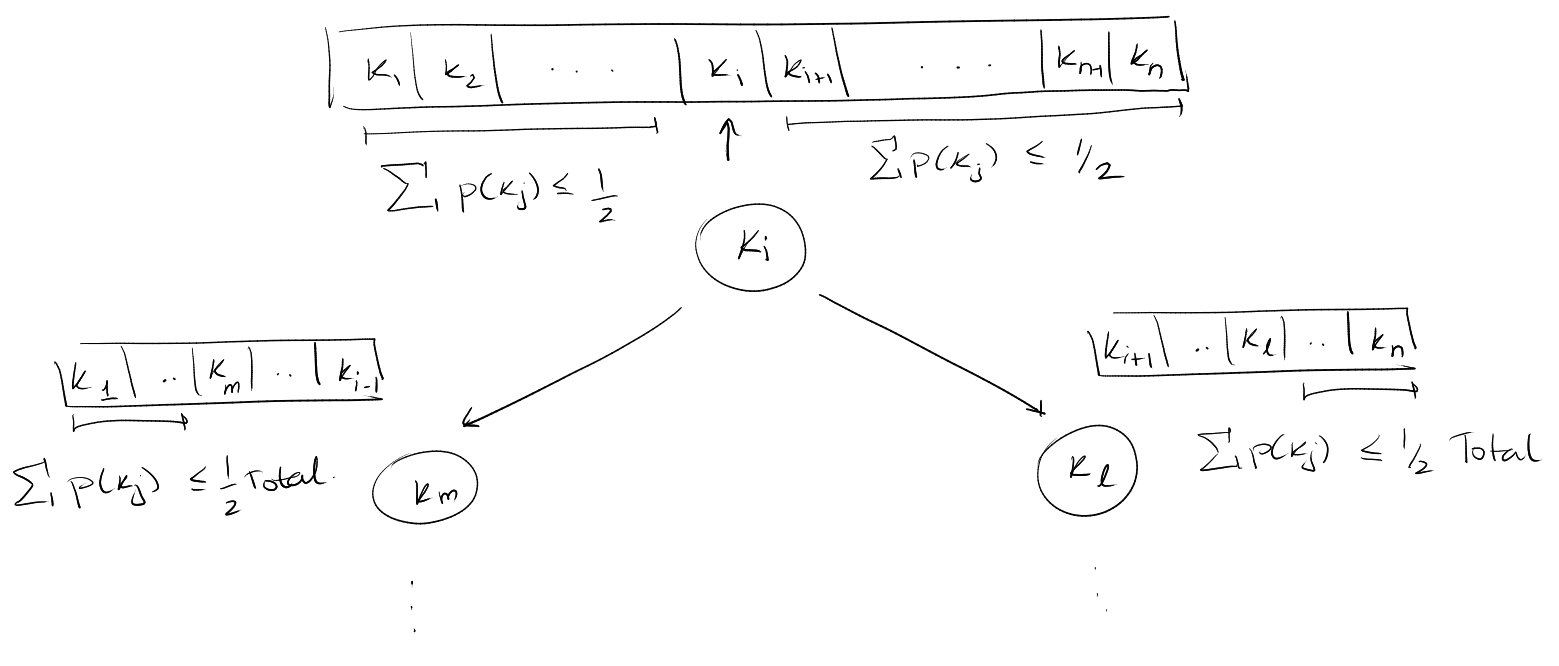
A common trick: Probability splitting.
We find a key \(k_i\) such that each side of the \(k_i\) the probability is less
than half the total probability of all the elements. At the root, the sum of all
probabilities is going to be \(1\), however, we use this recursively and the sum
will not be \(1\) at the different places.
\[
\begin{gather}
\sum_{j=1}^{i-1} p_j \leq \frac{1}{2} \sum_{j=1}^{n} p_j \\
\text{and} \\
\sum_{j=i+1}^{n} p_j \leq \frac{1}{2} \sum_{j=1}^{n} p_j \\
\end{gather}
\]
The key \(k_i\) becomes the root of a BST and then we do this recursively.
We're assuming we're given a sorted set of keys.
Observation: In \(T\), if node \(k_i\) has \(depth_T(k_i)\), then if we sum \(p_j\)
over all \(k_j \in T(k_i)\) where \(T(k_i)\) is the set of nodes in the sub-tree
rooted at \(k_i\):
\[
\sum_{k_j \in T(k_i)} p_j \leq \frac{1}{2^{depth_T(k_i)}}
\]
This follows since at each level we divide the nodes into two parts, the left
and the right sub-tree, in such a way that the sum of the probabilities is less
than half the total probability.
The tree \(T\) can answer queries in \(O(H+1)\) time.
Proof: We know
\[
\begin{gather}
p_i \leq \sum_{k_j \in T(k_i)} p_j \leq \frac{1}{2^{depth_T(k_i)}} \\
\text{and}\\
depth_T(k_i) \leq \lg \left(\frac{1}{p_i}\right)
\end{gather}
\]
Thus the expected depth of a key chosen is:
\[
\sum_{i=1}^{n} p_i \cdot depth_T(k_i) \leq \sum_{i=1}^{n} p_i \cdot \lg \left(\frac{1}{p_i} \right) = H
\]
To show that the tree can be constructed fast. To find the key \(k_i\) that holds
such a property. To find this key, we would require \(\Theta(n)\) time. This would
lead to an overall time of \(n^2\) similar to the other method to build a tree.
To speed this up, we calculate a prefix sums and stop at the point when sum is
over \(1/2\). Using this pre-calculated prefix sum array we can find all \(k_i\)
with the once calculated array using binary search. The total running time to
build the tree would therefore be \(\Theta(n \lg n)\).
But we can do even better: First we find \(k_i\) by doing a doubling search or an
exponential search.
- We calculate a prefix sum array.
- Check positions \(1, 2, 4, 8, \dots\) until we overshoot the expected prefix
sum.
- After we overshoot, we perform a binary search between the two elements.
Even though this is still \(\Theta(\lg n)\) or more accurately \(\Theta(\lg i)\)
(where \(i\) is the index found) it is actually preferable when we believe the key
is in the beginning of the list.
Therefore, we do this simultaneously from the beginning and the end. We start at
\(k_1\) and walking forward, and we also start at \(k_n\) and walk backward.
\(k_i\) can be found in \(O(\lg min(i, n-i+1))\). Then the total running time to
build the tree will be given by:
\[
T(n) = O(\lg min(i, n-i+1)) + T(i-1) + T(n-i)
\]
This works out to be \(O(n)\).
MTF Compression
We use the concept of entropy to bound the efficiency of compression
algorithms.
Elias Gamma Coding
Commonly used to code non-negative integers, whose max value is not known.
-
We first write down the binary representation of \(i\). The number of bits
needed would be \(\lfloor \lg i \rfloor + 1\) bits.
-
We prepend it by \(\lfloor \lg i \rfloor\) 0's.
Example: 9 -> 1001 -> 0001001.
When reading a sequence of bits, the number of zeros will tell us the number of
bits in the next number.
For the sequence: 9, 5, 7 we would encode it as 0001001 00101 00111.
The number of bits required to encode \(i\) would then be \(1 + 2 \lfloor \lg i
\rfloor\).
Better Than Elias Gamma Encoding
This is a scheme that uses fewer bits than the Elias Gamma Coding method by just
replacing the zeroes that prefix numbers with the Elias Gamma encoded number.
That is, the number of bits are encoded in unary which we can replace with the
Elias gamma encoding for that number.
Example: 9 -> 000 1001 -> 011 1001
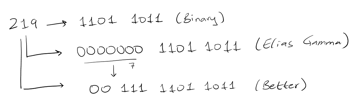
The number of bits required to encode \(i\) is now going to be \(1 + 2 \lfloor \lg
\lg i \lfloor\) bits to encode the length and then \(\lg i\) bits to encode the
number. Therefore the total required bits would be \(1 + 2 \lg \lg i + \lg i\)
bits. To summarize: \(\lg i + O(\lg \lg i)\).
We can do this recursively to get a slightly better encoding scheme. But we
don't need this. This is called recursive elias or elias omega codes.
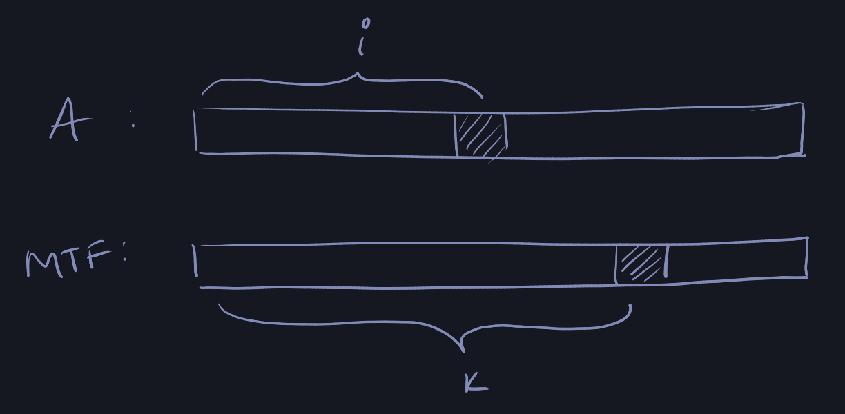
MTF Compression of encoding \(m\) integers from \(1, \dots, n\).
The sender and receiver each maintain identical lists containing integers \(1
\dots n\). To send the symbol \(j\), the sender looks for \(j\) in their list and
find it at position \(i\). The sender then encoding \(i\) using the 2 level Elias
Gamma encoding scheme and sends it to the receiver.
The receiver then decodes \(i\) and looks at the ith element in their list to find
\(j\). The sender and receiver both move element \(j\) to the front of their lists
and continue.
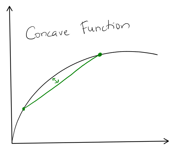
Jensen's Inequality:
Let \(f: R \to R\) be a strictly increasing concave function. Then the sum of all
\(f(t_i)\) for \(i \in [1, n]\) is subject to the constraint \(\sum t_i \leq m\) is
maximized when \(t_1 = t_2 = \dots = t_n = m/n\)
A concave function is a function such that between two points the curve is above
the line. \(f'\) is always decreasing.
The MTF compression algorithm compresses the sequence \(S_1, S_2, \dots, S_m\)
into \(n \lg n\) + \(mH\) + \(O(n \lg\lg n + m\lg H)\) bits.
Proof: If the number of distinct symbols between two consecutives occurances
of integers \(j\) is \(t-1\) then the cost of encoding the second \(j\) is \(\lg t +
O(\lg \lg t)\). This is because the element \(j\) would have moved to position
\(t\).
Therefore, the total cost of encoding all occurrences of \(j\) is
\[
C_j \leq \lg n + O(\lg \lg n) + \sum_{i=1}^{m_j} \left( \lg t_i + O(\lg \lg t_i) \right)
\]
since \(\sum t_i \leq m\)
\[
C_j \leq \lg n + O(\lg \lg n) + m_j (\lg \frac{m}{m_j}) + O(\lg \lg (\frac{m}{m_j}))
\]
Summing this over all \(j\), the total number of bits required:
\[
\sum_{j=1}^{n} C_j \leq n\lg n + O(n \lg \lg n) + mH + \sum_{j=1}^{m} O(m_j \lg
\lg \frac{m}{m_j})
\]
Here, \(p_j = m_j / m\), therefore we can replace the final sum in terms of
entropy.
\[
\text{Total cost} \leq n \lg n + mH + O(n \lg \lg n) + O(m \lg H)
\]
Here \(n\) is the size of the alphabet that we are encoding and \(m\) is the number
of elements in the sequence. \(mH\) is the theoretical lower bound. Therefore,
this solution gets pretty close to the theoretical lower bound.
Note: This assumes that symbols are purely independent from each other,
which is often not true. For example, the probability that you see "e" after the
letters "th" is not just 1 in 26 but a lot higher since "the" is a very frequent
word.
Gzip and Bzip2 compression uses the Barrow Wheeler Transformation compression
algorithms which offer a lot faster compression. Bzip2 uses BWT to transform the
data and then uses MTF with Huffman encoding.
Text Indexing Structures
We have an alphabet \(\Sigma\) with \(\sigma\) number of symbols. We are given a
text \(T\) of length \(n\) over the alphabet \(\Sigma\). We are required to search for
the pattern \(P\) of length \(p\) in text \(T\).
There are two separate approaches based on the situation.
If no preprocessing is allowed then we can't pre-construct a data structure to
help with answers queries. Then we need to use some sort of string matching
algorithms. The obvious approach leads to a running time of \(O(n \cdot p)\).
However, we can speed this up for a situation without preprocessing we can use
one of the following algorithms which do it in \(O(n + p)\):
- Knuth Morris Pratt
- Boyer-Moore
- Rabin-Karp
If we're allowed to use preprocessing and build data structures then we can
create text indexes to answers different queries for \(p\). The index speeds up
text search when each time a new pattern is given.
We are trading space for query time.
Warm Up Structure: Trie
- We represent a set of strings \(\{T_1, T_2, \dots, T_k\}\).
- A rooted tree with edges labelled with alphabets in \(\Sigma\).
- We represent strings as root to leaf paths in a trie, terminated with a new
letter.
We use an end of string symbol eg: $.
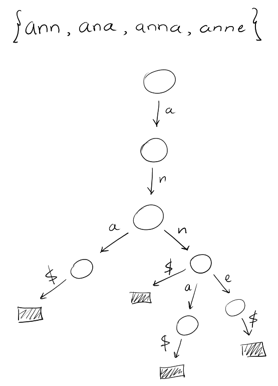
We sort the edges in lexicographic order.
An in-order traversal of the leaves then will get the strings in sorted order.
This is because we ordered the children of each node.
To check if \(p\) is in the set of strings \(\{T_1, T_2, \dots, T_k\}\) we can do a
top-down traversal. If each node stores pointers to each child in sorted order.
The number of nodes in the trie is \(n \leq \sum |T_i| + 1\).
Query time to check if \(p\) is in the trie: \(O(p \lg \sigma)\).
We see that there's a lot of space that's required by the nodes and therefore we
can compress the trie (compressed trie) for non-branching paths to a single
edge.
Suffix Trees
A compressed trie of all suffices of T$.
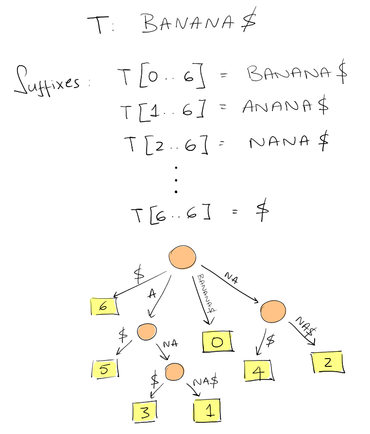
We have \(n+1\) leaves and each edge label is a substring \(T[i \dots j]\).
We only store two indices \(i, j\) to store the label of an edge.
The space required for this tree: \(O(n)\).
Text search for \(P\) gives a sub-tree whose leaves correspond to all occurrences
of \(P\). If we successfully use all characters of \(P\). If we have a mismatch then
\(T\) doesn't contain the substring \(P\).
If each node stores points to children then for a particular \(P\) the running
time would be \(O(p \lg \sigma)\). If we use perfect hashing time then the query
time goes down to \(O(p)\).
To find all occurrences of the substring requires running time: \(O(p + occ)\)
where \(occ\) is the number of occurrences of the pattern.
Applications:
- Longest repeated substring in \(T\): can be found by finding the branching node
with the maximum letter depth. This requires \(O(n)\) time.
However, for natural language the suffix tree requires around 15-20 times the
size of \(T\) to store the tree.
Suffix Arrays
We sort the suffixes of \(T\) and then we just store the starting indices.
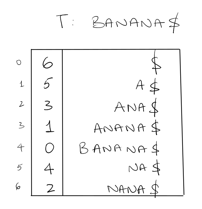
This requires \(n+1\) words. To search for a pattern \(P\) we can just perform a
simple binary search which would lead to a running time of \(O(p \lg n)\) to see
if \(P\) occurs in \(T\).
To find all occurrences of \(P\) in \(T\) would require \(O(p\lg n + occ)\).
A Simple Acceleration
Let \(L\) and \(R\) be the left and right boundaries of the current search interval. We
modify the binary search to use the midpoint to update \(L\) and \(R\) (normally, we
would update them to \(midpoint \pm 1\)).
Let \(l\) be the length of the longest prefix of \(T[SA[L] .. n]\) that matches
\(P\). Let \(r\) be the length of the longest prefix of \(T[SA[R] .. n]\) that
matches \(P\).
The initial values of \(l\) and \(r\) are obtained by direct comparison.
Here is an example search for the string "ABA":
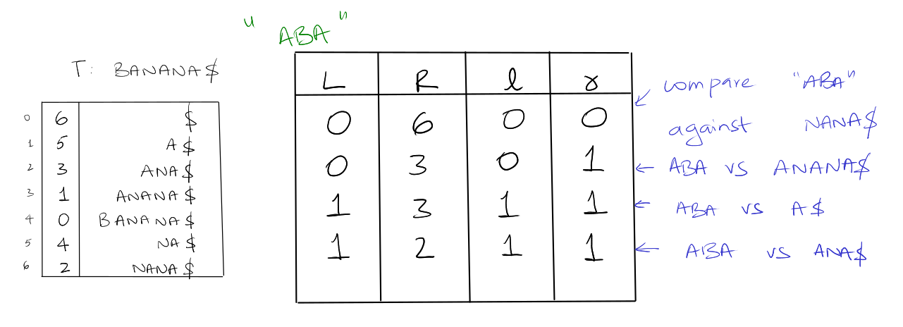
If there is a match at least one of them would be equal to the length of \(P\). \(h
= min(l, r)\).
Observation: first \(h\) characters of \(P\), \(T[SA(L) .. n]\), \(T[SA(L+1).. n]\),
\(\dots\), \(T[SA(R)..n]\) agree = \(P[0 .. h-1]\).
Since the first \(h\) characters are the same, we do not need to compare them, we
can just start from \(P[h]\). This way we are comparing fewer characters when
searching for the substring.
This approach doesn't change the theoretical upper bound but in practice speeds
up the search by quite a lot.
Super Accelerant
First we define a couple of terms:
- The longest common prefix of two string \(s_1\) and \(s_2\).
- \(lcp(i, j)\): gives t he length of the longest common prefix of \(T[SA(i)..n]\)
and \(T[SA(j)..n]\).
Call an examination of a character in \(P\) redundant if that character has been
examined before.
Goal: Reduce the number of redundant character examinations to at most 1 per
iteration of the binary search. This would lead to a running time of \(O(\lg n)\)
for the binary search. In turn leading to a time of \(O(p + \lg n)\).
To achieve this, we perform a little more preprocessing: for each triple \((L, M,
R)\) that can possibly arise during the binary search we pre-compute \(lcp(L, M)\)
and \(lcp(M, R)\).
There are \((n+1)-2 = n - 1\) triples in total. We never use \(0\) or \(n\) as a value
of \(M\) since it is always a midway point.
The total extra space required to build this table is \(2n-2\).
Let \(Pos(i)\): be the suffix that corresponds to the \(i\)th entry of the suffix
array: \(T[SA[i] .. n]\).
Case 1:
If any iteration of the binary search if \(l=r\) then compare \(p\) to suffix
\(Pos(M)\), starting from \(P[h]\). Since the first \(h\) characters match, we don't
need to compare those again.
Case 2 (a):
If \(l \neq r\), assume that \(l > r\) without loss of generality (just a symmetric
case).
If \(lcp(L, M) > l\) then we have a situation where the \(L\) and \(M\) strings agree
with each other more than \(L\) agrees with \(P\).
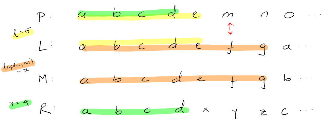
Since \(P > L\) and \(lcp(L, M) > l\), therefore \(P > Pos(M)\). Therefore, no
examination is of \(P\) is needed. \(L \gets M\) and \(l\) and \(r\) don't change.
Case 2 (b):
If \(l \neq r\), assume that \(l > r\) without loss of generality (just a symmetric
case).
If \(lcp(L, M) < l\) we have a situation where \(L\) and \(M\) agree less than \(L\)
agrees with \(P\).
Since \(P > L\) and \(lcp(L, M) < l\), therefore \(P < Pos(M)\). Rational: \(P[h-1] =
L[h-1]\) but \(L[h-1] < M[h-1]\). Therefore, \(R \gets M\), \(r \gets lcp(L, M)\) and
\(l\) remains unchanged.
Case 2 (c):
If \(l \neq r\), assume that \(l > r\) without loss of generality (just a symmetric
case).
If \(lcp(L, M) = l\) we have a situation where \(L\), \(M\), and \(P\) all agree the
same amount of characters. Therefore \(P\) agrees with \(Pos(M)\) up to position
\(l-1\). We start the comparison from position \(P[l]\).
Running Time Analysis
The two cases in which the algorithm examines the character during the
iterations, the comparison starts with \(P[max(l, r)]\); suppose \(k\) characters
were examined for one iteration, then there are \(k-1\) matches and \(max(l, r)\)
increases by \(k-1\). Hence, at the start of any iteration, \(P[max(l, r)]\) may
have been examined, but the next character has not been.
Therefore, we have reduced the number of redundant comparisons to at most 1 per
iteration.
From this, we get a running time for the entire search to be \(O(\lg n + p)\).
Construction Time
Suffix trees / arrays for string over a constant sized alphabet can be
constructed in \(O(n)\) time. Trees and arrays for strings over alphabets \(\Sigma
= \{1, 2, \dots, n\}\) can also be constructed in \(O(n)\) time.
Succinct Data Structures
Succinct Trees
Number Of Possible Trees
First we calculate the number of possibles trees with \(n\) nodes.
For binary trees, the Catalan number is the number of trees possible for \(n\)
nodes. \(C_n = \binom{2n}{n} / (n + 1)\) where \(\binom{2n}{n}\) is \(2n\) choose \(n\).
For ordinal trees, trees with numbered children (1st, 2nd, ...), can be mapped
to a binary tree, the left child of a node would be the first child in the
ordinal tree. The right child is the immediate right sibling.
Left child (binary tree) -> first child (ordinal tree) and right child (binary
tree) -> immediate right sibling (ordinal tree).
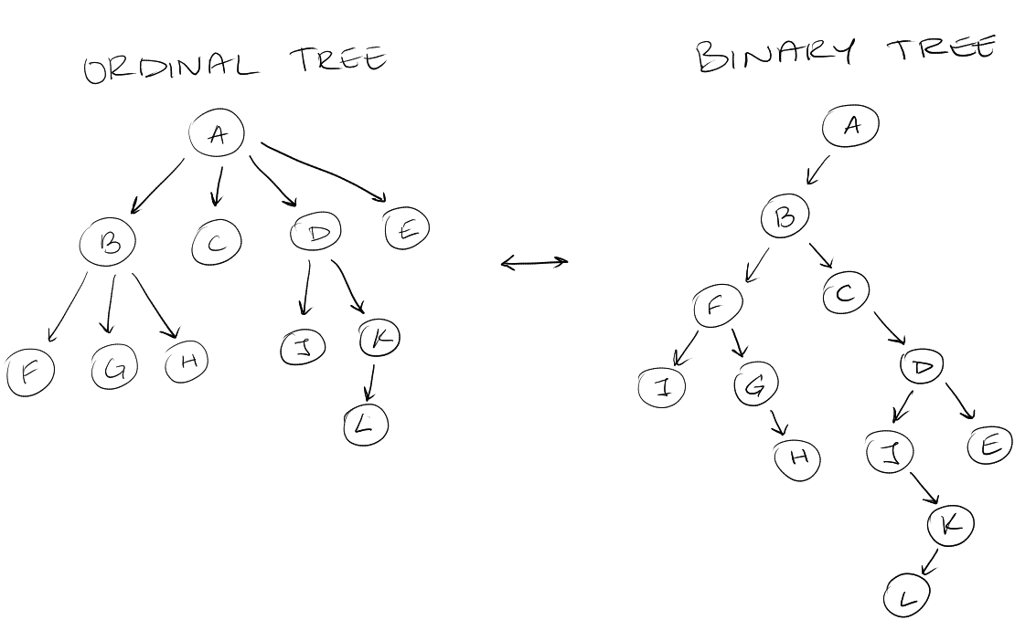
Note that since the root of the ordinal tree isn't going to have an immediate
right sibling, the root of the binary tree is always going to have no right
child. To convert a binary tree to an ordinal tree, we need to add a dummy root
to ensure it doesn't have a right child.
From this conversion we see that the number of ordinal trees is \(C_{n-1}\) for
\(n\) nodes.
Now we find the information theoretic lower bound of representing a binary tree.
A combinational object of \(n\) elements with \(u\) being the number of different
such objects of size \(n\): the lower bound for such an object is \(\lg u\) bits.
For binary trees:
\[
\begin{align}
\lg C_n &= \lg \left( \frac{2n!}{n!^2} \right) - \lg(n+1) \\
&= \lg (2n!) - 2\lg(n!) - \lg (n+1) \\
\text{(Using }& \text{Stirling's Approximation)} \\
&= 2n \lg(2n) - 2n\lg(n) + o(n) \\
&= 2n(1 + \lg n) - 2n \lg n + o(n) \\
&= 2n + o(n)
\end{align}
\]
More careful analysis leads to a bound of:
\[
\lg C_n \approx 2n - \frac32 \lg n + O(1)
\]
Level Order Representation
-
Append external nodes \((\square)\) for each missing child so that we form a
complete binary tree.
-
For each node in the level-order we write a \(0\) if it is external or \(1\) if
it is internal.
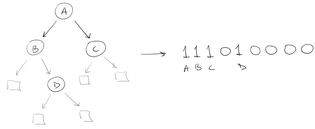
This requires \(2n + 1\) bits of space.
We can navigate the tree in the following way: The left and right children of
the \(i\)th internal node are at positions \(2i\) and \(2i+1\) in the bit vector.
Proof: Induction
Clearly, tree for \(i=1\)
For \(i>1\), by the induction hypothesis, the children of the \(i-1\)st internal
node are at \(2(i-1)\) and \(2(i-1)+1\) positions. There are two cases, if \((i-1)\)st
and \(i\)th nodes are on the same level.
Level ordering is preserved in the children. That is, \(A\)'s children precedes
\(B\)'s children if and only if \(A\) precedes \(B\). All nodes between \((i-1)\)st
internal node and the \(i\)th internal node are external nodes, with no children.
So, the children of the \(i\)th internal node immediately follow the children of
the \((i-1)\)th internal node, at positions \(2i\) and \(2i+1\).
Rank And Select in Bit Vectors
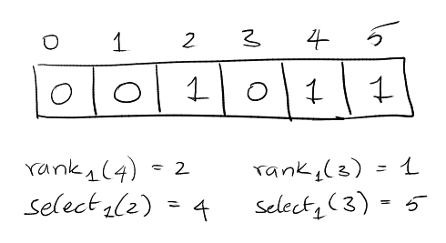
If we identify each node by its position in the bit vector:
left_child(i): \(2 \cdot rank_1(i)\)right_child(i): \(2 \cdot rank_1(i) + 1\)parent(i): \(select_1(\lfloor i/2 \rfloor)\)
Rank
The object is to get the rank operation to work in \(O(1)\) running time.
We split the bit vector into \(\lg ^2 n\) bit super-blocks. For each super-block
we store the cumulative rank each of which will require \(\lg (n)\) bits to store.
The total space required for this additional information is going to be:
\[
O(\frac{n}{\lg ^2 n} \cdot \lg n) = O(\frac{n}{\lg n}) bits
\]
Then we split each super-block into \(1/2 \lg n\) bit blocks. We store the
cumulative rank within the super block. This requires \(O(\lg \lg n)\) more space
per super block.
\[
O(\frac{n}{\lg n} \cdot \lg \lg n) = o(n) bits
\]
We use a lookup table for bit vectors of length \(1/2 \lg n\), i.e. for any
possible bit vector of length \(1/2 \lg n\) and for each of its positions we store
the rank of that position.
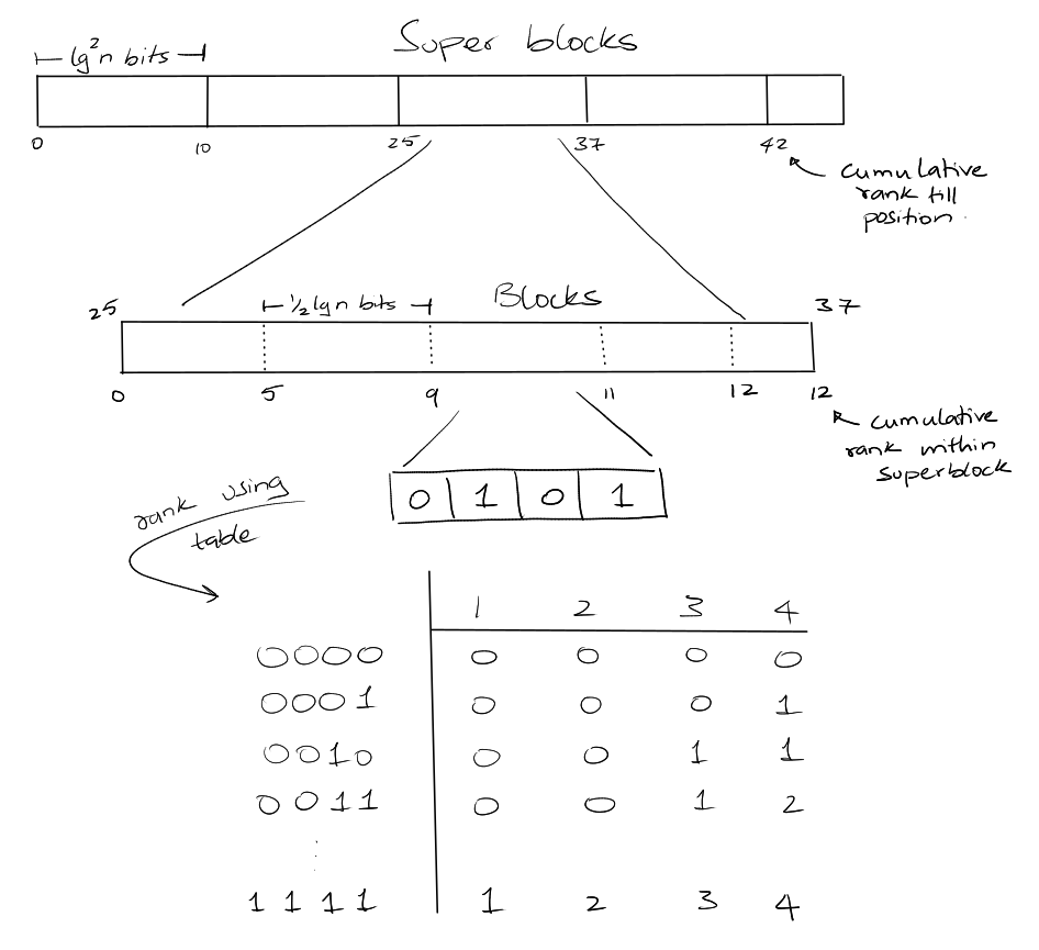
Look up in this 2D table. There are \(\sqrt{n}\) bit vectors of length \(1/2 \lg
n\). This requires the space of:
\[
O(\sqrt{n} \lg n \lg \lg n)
\]
Where \(\sqrt{n}\) is the rows in the table, \(\lg n\) is the number of columns, and
\(\lg \lg n\) is the number of bits required to store the answer.
The overall space for this structure:
\[
O(\frac{n \lg \lg n}{\lg n})
\]
We retrieve the rank of a position using exactly 3 steps (\(O(1)\)):
- Find the rank of the super-block containing it.
- Find the relative rank within the super-block and add it.
- Find the relative rank of the element within the block using the lookup
table and add it.
The best way to get rank in \(O(1)\) time can be reduced to \(O(n / \lg^k n)\) bits
for any \(k = O(1)\).
Select
This uses a similar idea for bit more involved. Here is a reference paper that
does the select operation in \(O(1)\) time.
Reference paper for rank and
select
Binary Tree Bit Vector Summary
We can store the binary tree using \(2n + o(n)\) bits and the support left child,
right child, and parent in \(O(1)\) running time.
Binary Trees Using Balanced Parenthesis Repr.
If we want to represent a binary tree then we first need to convert it to an
ordinal tree before we do the balanced parenthesis representation. This is the
same process an demonstrated above but here is another example. Note that we use
the dummy node as the parent node for the ordinal tree.

- We perform a DFS and the first time we visit a node we append a
(.
- When we visit it after visiting all its descendants we append a
).
For the above tree, the balanced parenthesis representation would look like:
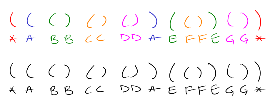
There are exactly \(2n\) parenthesis.
| Binary Tree |
Ordinal Tree |
Parenthesis Representation |
| Node |
Node |
Left paren and matching right paren |
| Left child |
First child |
Next character '(' => child |
| Right child |
Next sibling |
First char after matching closing paren |
| Parent |
Prev sib / Parent |
Prev Char '(' => parent, ')' => prev sibling |
|
Sub tree size |
half count between matching parenthesis |
| Sub tree size |
|
size(node) + size(siblings) |
A bit vector with match parenthesis takes \(O(1)\) time, with \(O(n)\) bits space.
The total space required would be \(2n + o(n)\) bits since we still need to
support rank and select.
Outer Planar Graphs
An adjacency matrix representation of a graph requires \(O(n^2)\) bits and an
adjacency list representation requires \(O(E + V)\) words.
An outer planar graph is a graph such that if all the nodes are drawn in a line,
their connections all lie on one side and the edges do not cross.
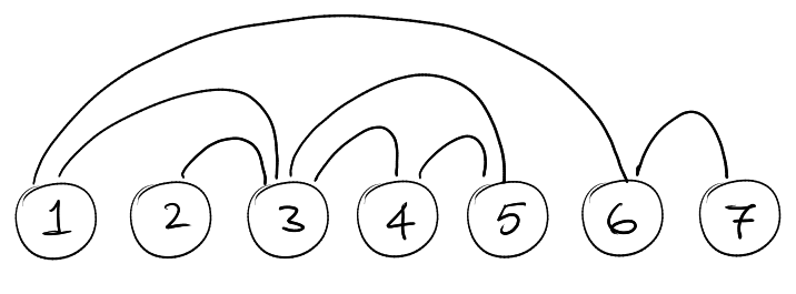
We require two data structures to represent this graph:
-
\(B\): A bit vector. If a node has degree \(d\) then we store 1 followed by \(d\)
zeroes.
-
\(P\): Parenthesis representation string. ) if edge incident to node to left,
otherwise (.
For the above graph we would have the following representation:
B: 1000 100 10 10 ...
P: (((  )(  (  )  ...
- The
degree(x) is given by select(x+1) - select(x) - 1.
- The
neighbours(x) is given by locating the 0s corresponding to edges
incident on x. select(x) + 1 ..., select(x+1) - 1
For each edge we need to find the other endpoint by parenthesis matching.
neighbours(2): 1, 5, 3. This requires \(O(d(x))\) running time.
For Adjacency(x, y) with the requirement that \(x \leq y\) we perform the
following steps:
- Find the matching parenthesis of the first
( corresponding to \(x\).
- If the position is before \(y\), then its false.
- If position is \(y\) then true.
- If position is \(>\) all edges of \(y\) finding matching opening parenthesis of
last closing parenthesis corresponds to \(y\). If this hits \(x\) then we return
true otherwise false.
This operation can be done using rank and select and requires a running time
of \(O(1)\).
The total space required by this structure is then $n + 4m +o(/static/uploaded-data/f3eba584-5ec4-4e8f-b8cb-d06ea8e498a0.png