Acknowledgement
These notes are based on the slides provided by the professor, Qiang Ye, for the
class "CSCI-3120 Operating Systems". I am taking/took this class in Fall
2023-2024 semester. If there are corrections or issues with the notes, please
use the contact page to let me know. A lot of the words and images are either
directly taken from the slides or have been paraphrased slightly.
CH1: Introduction
Definitions of "Operating System":
- Everything a vendor ships when you order an operating system.
- The one program running at all times on the computer.
- Actually, it is the kernel part of the operating system.
- Everything else is either system program or application program.
Computer Architecture
Computer Architecture: Logical aspects of system implementation as seen by
the programmer. Answers the question: "How to design a computer?".
Computer Organization: Deals with all physical aspects of computer systems.
Answers the question: "How to implement the design?".
Multiprocessor Systems
Symmetric Multiprocessing (SMP)
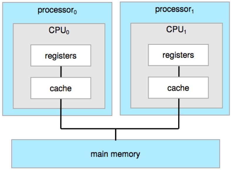
Each CPU processor performs all kinds of tasks, including operating-system
functions and user processes.
Multicore Systems
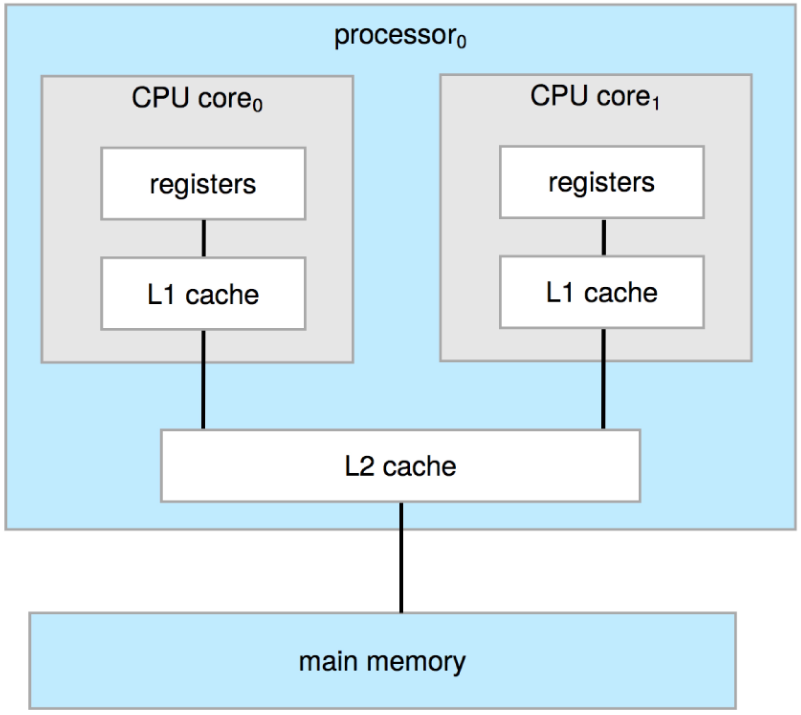
Multicore systems are systems in which multiple computing cores reside on a
single chip. Multicore systems can be more efficient than systems with multiple
processors because on-chip communication between cores is faster than
between-chip communication.
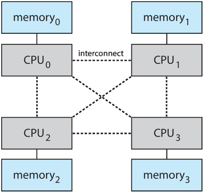
An approach to share memory is to provide each CPU (or group of CPUs) with their
own local memory that is accessed via a local bus.
Clustered Systems
Clustered systems differ from the multiprocessor systems in that they are
composed of two or more individual systems. Each individual system is typically
a multicore computer. Such systems are considered loosely coupled.
Computer Organization
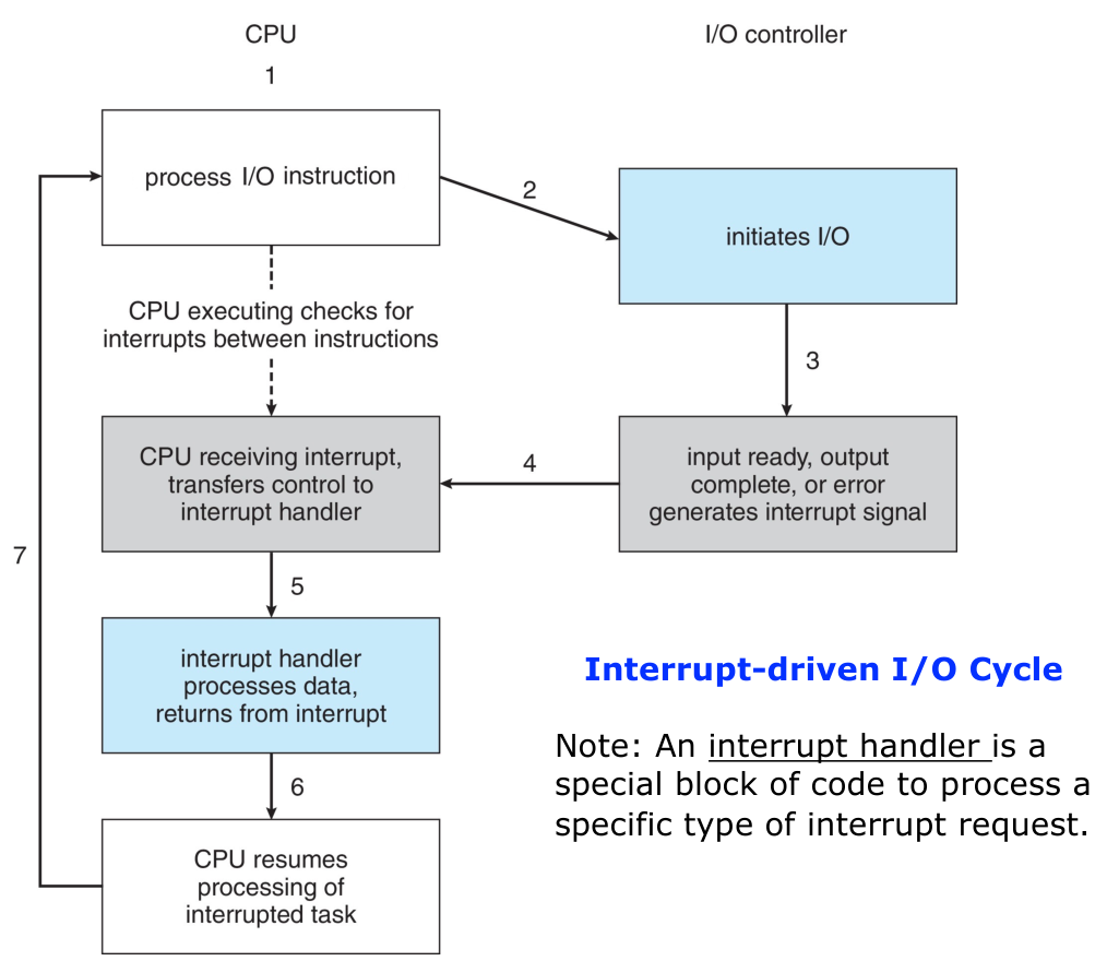
Interrupts
An interrupt is a signal to the processor emitted by hardware or software
indicating an event that needs immediate attention.
Two types of interrupts:
- Hardware Interrupts: defined at the hardware level.
- Software Interrupts: also known as trap or exception defined at the OS
level.
Operating System Operations
Bootstrap Program
When a computer starts, it needs to run an initial program to find the operating
system which then needs to be loaded. This initial program is known as
bootstrap program, tends to be simple. It initializes all aspects of the
system, from CPU registers to device controllers to memory contents. In
addition, it loads the operating-system kernel into memory. Thereafter, the OS
will take over the system.
- Power On: User turns on the computer.
- BIOS/UEFI Initialization: Basic Input/Output System (BIOS) or Unified
Extensible Firmware Interface (UEFI) starts.
- POST: Hardware check via Power-On self-test.
- Bootstrap Program Loaded: Small program that starts the boot sequence.
- Bootloader Activated: Loads and stars the operating system's kernel.
- OS Kernel Loaded: Core of the operating system is loaded into memory.
- OS Initialization: Operating system is initialized and becomes fully
operational.
Multiprogramming
The operating systems keeps several processes in memory simultaneously. The
operating system picks and begins to execute one of these processes at a time.
Eventually, the process may have to wait for some task such as I/O operation to
complete. When this event occurs, the operating system simply switches to and
executes another process.
Multitasking
Multiprogramming doesn't give any guarantee that a program will run in a timely
manner. The very first program may run for hours without needing to wait.
Multitasking is logical extension of multiprogramming where the CPU executes
multiple processes by switching among them, but the switches occur more
frequently, providing the user with a fast response time.
Multimode Operation
The operating system is responsible to ensure that hardware and software
resources of the computer system are protected from incorrect or malicious
programs including the operating system itself.
In order to ensure the proper execution of system, we must be able to
distinguish the execution of operating-system code and user-defined code. The
approach taken by most computer systems is to provide hardware support that
allows differentiation of various modes of execution.
At the least, a system must have a kernel mode (supervisor mode, privileged
mode, system mode) and a user mode. A bit, called the mode bit is added
to the hardware of the computer to indicate the current mode.
If an attempt is made to execute a privileged instruction in user mode, the
hardware does not execute the instruction. Instead, it treats it as an illegal
instruction.
-
Intel processors have 4 separate protection rings, where ring 0 is
kernel mode and ring 3 is user mode. The other modes are for things such as
hypervisors.
-
ARM v8 systems have 7 modes.
-
CPUs that support virtualisation frequently have a separate mode to
indicate when the virtual machine manager (VMM) is in control of the system.
In this mode, the VMM has more privileges than user processes but fewer than
the kernel.
History of Free Operating Systems
In the early days of modern computing (1950s), software generally came with
source code. However, companies sought to limit the use of their software to
paying customers. To counter the move to limit software use and redistribution,
in 1984, Richard Stallman started developing a free, UNIX-compatible operating
system called GNU, which is a recursive acronym for "GNU's Not Unix".
Four Essential Freedoms
The Free Software Foundation (FSF) was founded to support the free-software
movement. This was a social movement with the goal of guaranteeing four
essential freedoms for software users.
- The freedom to run the program.
- The freedom to study and change the source code.
- The freedom to redistribute copies.
- The freedom to distribute copies of the modified versions.
CH2: Operating System Structures
Services
Operating systems provide a collection of services to programs and users. These
are functions that are helpful to the user.
These are some areas where functions are provided:
- User Interface
- Program execution
- I/O operations
- File-system manipulation
- Communications (IPC)
- Error detection.
Another set of OS functions exist to ensure the efficient operation of the
system itself.
- Resource allocation: CPU, Memory, file storage etc.
- Accounting: Logging, tracking.
- Protection and Security: Owners managed and maintained.
User Interfaces
Command-Line Interface (CLI)
The command-line interface (a.k.a. command interpreter) allows direct command
entry. The CLI fetches a command from the user and executes it.
There are two types of commands:
- Built-in commands: These are a part of the CLI program.
- External commands: These commands correspond to independent programs.
You can check if a command is a built-in or an external using the type
built-in command.
$ type type
type is a shell builtin

$ type cd
cd is a shell builtin

$ type cat
cat is /usr/bin/cat
System Calls
System calls provide an interface to services made available by an operating
system. System calls are generally available as functions written in C and C++.
Certain low-level tasks may have to be written using assembly-language
instructions.
However, most programmers do not use system calls directly. Typically,
application developers design programs according to a high-level API. The API
specifies a set of functions that are available to an application programmer.
Example: read and write functions in C (using the stdio library) are
actually wrappers around the corresponding read and write system calls.
Types of System Calls
- Process control
- create/terminate process
- load/execute process
- get/set process attributes
- wait/signal events
- allocate and free memory.
- File management
- create/delete files
- open/close files
- read/write/reposition file
- get/set file attributes.
- Device management
- request/release device
- read, write, reposition
- get/set device attributes
- logically attach or detach devices.
- Information maintenance
- get/set time, date
- get/set system data.
- Communications
- create/delete communication connection
- send/receive messages
- transfer status information
- attach/detach remote devices.
- Protection
- get/set file permissions
- allow/deny user access.
The following table illustrates various equivalent system calls for Windows and
UNIX operating systems.
| Category |
Windows |
Unix |
| Process control |
CreateProcess() |
fork() |
| ExitProcess() |
exit() |
| WaitForSingleObject() |
wait() |
| File management |
CreateFile() |
open() |
| ReadFile() |
read() |
| WriteFile() |
write() |
| CloseHandle() |
close() |
| Device management |
SetConsoleMode() |
ioctl() |
| ReadConsole() |
read() |
| WriteConsole() |
write() |
| Information maintenance |
GetCurrentProcessID() |
getpid() |
| SetTimer() |
alarm() |
| Sleep() |
sleep() |
| Communications |
CreatePipe() |
pipe() |
| CreateFileMapping() |
shm_open() |
| MapViewOfFile() |
mmap() |
| Protection |
SetFileSecurity() |
chmod() |
| InitializeSecurityDescriptor() |
umask() |
| SetSecurityDescriptor() |
chown() |
Compiler, Linker, and Loader
-
Compiler: Source code needs to be compiled into object files. Object files
are designed to be loaded into any physical memory location.
-
Linker: Linker combines object codes into a binary executable file. If the
object code corresponding to a library is needed, the library code is also
linked into the executable file.
-
Loader: Executable files must be brought into memory by the loader to be
executed.
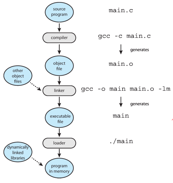
This is statically linking the libraries to the program. However, most systems
allow a program to dynamically link libraries as the program is loaded. Windows,
for instance, supports dynamically linked libraries (DLLs).
The benefit of this approach is that it avoids linking and loading libraries
that may end up not being used by an executable file. Instead, the library is
conditionally linked and is loaded if it is required during program run time.
Aside on Dynamic Libraries
Dynamically Linked Libraries (DLLs) on windows and shared libraries (on UNIX)
are kinda-sorta the same thing. The are loaded on requirement into the program
when the program requires it.
The main advantage of shared libraries is the reduction of used memory (in my
opinion). Since it's the same library that is loaded into multiple programs, if
a program has already loaded a library, then a new program that requires it is
only given a mapping to it and the memory is not actually copied. This means
that each program THINK it has a separate copy of the library but the in memory
there is only one copy of it. So functions like printf or read, that are
used a lot, are only loaded into memory ONCE rather than a few hundred times.
Object files and executable files typically have standard formats that include:
- The compiled machine code
- A symbol table containing metadata about functions
- Variables that are references in the program.
For UNIX/Linux systems, this standard format is known as Executable and
Linkable Format (ELF). Windows systems use the Portable Executable (PE)
format. MacOS uses the Mach-O format.
Operating System Design
- User goals: operating system should be convenient to use, easy to learn,
reliable, safe, and fast.
- System goals: operating system should be easy to design, implement, and
maintain, as well as flexible, reliable, error-free, and efficient.
Operating System Structure
A system as large and complex as a modern operating system must be engineered
carefully. A common approach is to partition the task into small components.
Each of these modules should be a well-defined portion of the system, with
carefully defined interfaces and functions.
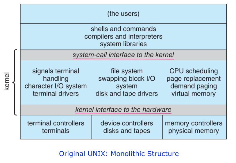
Monolithic Structure
The simplest structure for organizing an operating system is no structure at
all. That is, place ll the functionality of the kernel into a single, static
binary file that runs in a single address space.
An example of this type of structure is the original UNIX operating system,
which consists of two separable parts: Kernel, System programs.
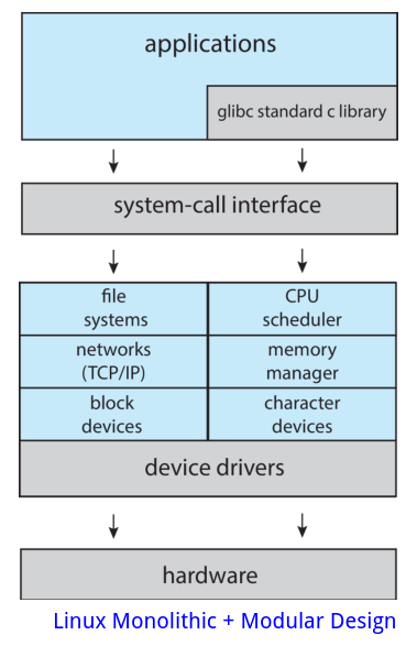
The Linux operating system is based on UNIX and is structured similarly, as
shown in the below figure. Applications typically use the standard C library
(note that the standard C on Linux is called glibc) when communicating with
the system call interface to the kernel.
The Linux kernel is monolithic in that it runs entirely in kernel mode in a
single address space. However, it does have a modular design that allows the
kernel to be modified during run time. This is discussed in a later section.
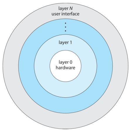
Layered Structure
-
The operating system is divided into a number of layers (levels), each built
on top of lower layers.
-
The bottom layer (layer 0), is the hardware; the highest (layer N) is the user
interface.
-
With modularity, layers are selected such that each layer only uses functions
and services provided by the layer immediately below it.
Microkernel Structure
- As UNIX expanded, the kernel became large and difficult to manage.
- In 1980s researchers at Carnegie Mellon University developed an operating
system called "Mach" that modularized the kernel using the microkernel
approach.
- This method structures the operating system by:
- removing all non-essential components from the kernel
- implementing the non-essential components as user-level programs that
reside in separate address spaces, which results in a smaller kernel.
- Typically, microkernels provide minimal:
- process management (i.e. CPU scheduling)
- memory management
- communications (IPC).
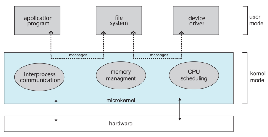
The main function of microkernel is to provide communication between the client
program and the various services that are also running in user space.
Communication is provided through message passing.
The performance of microkernels can suffer due to increased overhead. When two
user-level services must communicate, messages must be copied between the
services, which reside in separate address spaces. In addition, the operating
system may have to switch from one process to the next to exchange the messages.
The overhead involved in copying messages and switching between processes has
been the largest impediment to the growth of microkernel-based operating
systems.
Modular Structure
Perhaps the best current methodology for operating-system design involves using
loadable kernel modules (LKMs). The kernel has a set of core components and
can link in additional services via modules, either at boot or during run time.
This type of design is common in modern implementations of UNIX (such as Linux,
MacOS, and Solaris) as well as Windows.
The modular structure resembles the layered structure in that each kernel
section has defined, protected interfaces. However, modular structure is more
flexible than a layered system, because any module can call any other module.
Hybrid Structure
Most modern systems do not follow any strictly-defined structure. Instead, they
adopt the hybrid structure, which combines multiple approaches to address
performance, security, usability issues.
Examples:
Linux is monolithic, because having the operating system in a single address
space provides very efficient performance. However, it is also modular, so that
new functionality can be dynamically added to the kernel.
Building and Booting Linux
Here's a guide to building the Linux kernel yourself.
- Download Linux source code (https://www.kernel.org).
- Configure kernel using the command
make menuconfig.
- This step generates the
.config configuration file.
- Compile the main kernel using the command
make.
- The make command compiles the kernel based on the configuration parameters
identified in the
.config file, producing the file vmlinuz, which is
the kernel image.
- Compile kernel modules using the command
make modules.
- Just as with compiling the kernel, module compilation depends on the
configuration parameters specified in the
.config file.
- Install kernel modules into
vmlinuz using the command make modules_install.
- Install new kernel on the system using the command
make install.
- When the system reboots, it will begin running this new operating systems.
System Boot
BIOS
For legacy computers, the first step in the booting process is based on the
Basic Input/Output System (BIOS), a small boot loader.
Originally, BIOS was stored in a ROM chip on the motherboard. In modern
computers, BIOS is stored on flask memory on the motherboard so that it an be
rewritten without removing the chip from the motherboard.
- When the computer is first powered on, the BIOS is executed.
- This initial boot loader usually does nothing more than loading a second boot
loader, which is typically located at a fixed disk location called the boot
block. Typically, the second boot loader is a simple program and only knows
the address and the length of the remainder of the bootstrap program.
- In the typical scenario, the remainder of the bootstrap program is executed
to locate the OS kernel.
UEFI
For recent computers, the booting process is based on the Unified Extensible
Firmware Interface (UEFI).
UEFI has several advantages over BIOS:
- Better support for larger disks (over 2TB)
- Flexible pre-OS environment: UEFI can support remote diagnostics and repair
computers, even with no operating system installed.
Details found here:
wikipedia
CH3: Processes
Modern computer systems allow multiple programs to be loaded into memory and
executed concurrently. Formally, a process is a program in execute.
A process has a layout in memory that looks like the following diagram:
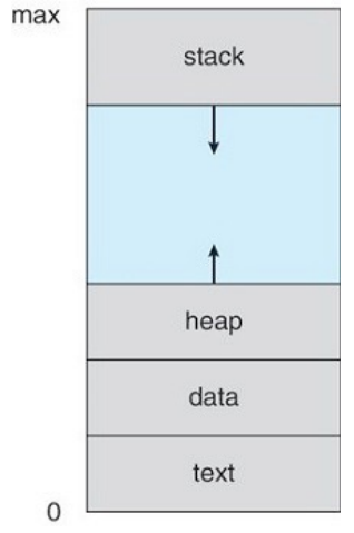
- Text: Contains executable code.
- Data: Global variables.
- Heap: Memory that is dynamically allocated during runtime.
- Stack: Temporary data storage when functions are invoked.
The text and data sections are fixed as their sizes do not change during
program run time. The stack and heap however, can grow and shrink
dynamically during the program execution.
Each time a function is called, an activation record containing function
parameters, local variables, and the return address is pushed onto the stack;
when control is returned from the function, the activation record is popped from
the stack.
Memory Layout of a C program
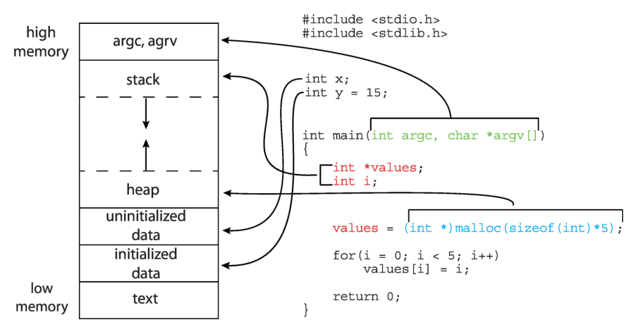
- The data section is divided into two sub-sections: initialized and
uninitialized data.
- A separate section is provided for the
argc and argv parameters passed to
the main() function from the operating system.
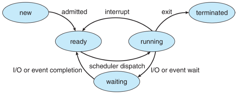
Process State
As a process executes, it can change state. The state of a process is defined in
part by the activity of that process.
The possible states a process can be in:
- New: The process is created.
- Running: Instructions in the process are being executed.
- Waiting: The process is waiting for some event to occur.
- Ready: The process is waiting to be assigned to a processor.
- Terminated: The process has been terminated.
Note that the state names are generic and they vary across operating systems.
Process Control Block
The Process Control Block (PCB), also known as Task Controlling Block (TCB), is
a data structure in the OS kernel, which contains the information needed to
manage the scheduling of a process.
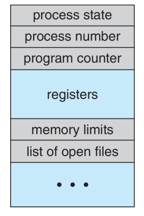
- State: state of the process.
- Number: process ID.
- Program counter: location of instruction to execute.
- CPU registers: contents of all process-related registers.
- CPU scheduling information: process priority, points to queues etc.
- Memory management information: memory allocated to the process.
- Accounting information: CPU used, clock time elapsed since state, time limits.
- IO status information: I/O devices allocated to process, list of open files, etc.
Scheduling
In a computer running concurrent processes, the OS needs to schedule processes
effectively. The number of processes currently in memory is known as the
degree of multiprogramming.
Most processes can be described as either I/O bound (spends most of its time
doing I/O operations) or CPU bound (spends most of its time doing
computations).
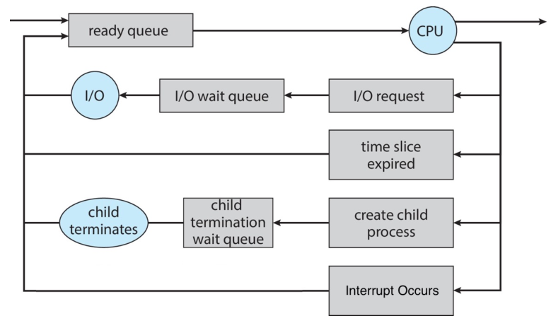
To schedule processes effectively, an OS typically maintains multiple scheduling
queues, such as the ready queue and the wait queue.
-
Ready queue: a set of processes residing in main memory, ready and waiting
to be executed.
-
Wait queue: a set of processes waiting for an event (e.g. I/O).

Here is an example of a queueing diagram:
CPU Scheduler
The role of the CPU scheduler is to select a process from the processes in
the ready queue and allocate a CPU core to the selected one. To be fair to all
processes and guarantee timely interaction with users, the CPU scheduler must
select a new process for the CPU frequently.
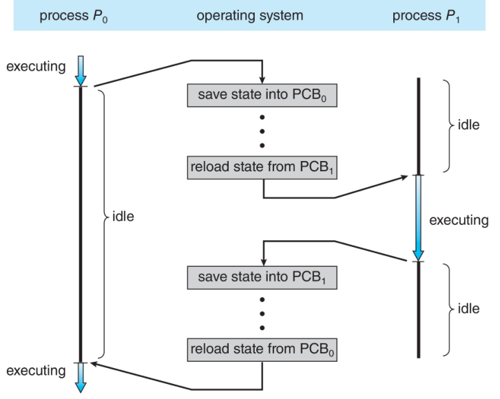
Context Switching
Switching the CPU core to another process requires performing a state save of
the current process and a state restore of a different process. This task is
known as a context switch. When a context switch occurs, the kernel saves
the context of the old process in its PCB and loads the saved context of the new
process.
Context switch time is overhead, because the system does not do useful work
while switching. Switching speed varies from machine to machine, depending on
memory speed, number of registers etc. Typically, it takes several microseconds.
Process Creation
The OS needs to provide mechanisms for process creation and process termination.
The creating process is called a parent process, and the created process is
called the child process of the parent process.
A child process may in turn create other processes, forming a tree of
processes.
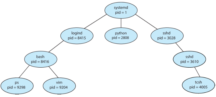
The figure above is a typical tree of processes for the Linux operating system,
showing the name of each process and its pid. Most operating systems identify
each process using a unique process identifier (pid), which is typically an
integer number.
The systemd process (init on Arch Linux) always has a pid of 1 and servers
as the root process for all user processes, and is the first user process
created when the system boots.
When a process creates a new process, two possibilities exist for its execution:
- The parent continues to execute concurrently with the children.
- The parent waits till some or all of its children have terminated.
There are also two address-space possibilities for the new process:
- The child process is a duplicate of the parent process, it has the same
data as the parent (see note under for more details).
- The child process has a new program loaded into itself.
NOTE (Additional details): When a child process is created on Linux, the OS
maps the same physical memory of the process to two separate processes. Although
each process THINKS they have an identical but separate copy of the data, the
data is only stored once. However, if there is a write operation performed on
the data, then that data that was written to is first copied to have separate
physical versions. Linux follows the "copy-on-write" principle
(https://en.wikipedia.org/wiki/Copy-on-write).
Creating Processes On Unix
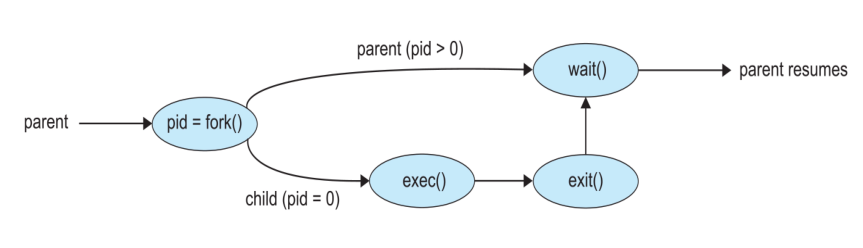
On Unix, a child process is created by the fork() system call. The parent and
child process continue to be executed and the next instruction is the one right
after the fork(), with one difference: The return code for the fork() is
zero for the child process and is a positive process identifier of the child for
the parent process. If fork() leads to a failure, it return -1.
- Parent:
fork() returns child process ID.
- Child:
fork() returns 0.
After a fork() system call, the child process can use one of the exec()
family of system calls to replace the process's memory space with a new program.
After a fork() the parent cal issue a wait() system call to move itself to
the wait queue till the termination of the child.
When the child terminates, the wait() system call in the parent process is
completed and the parent process resumes its execution.
Process Creation In C
#include <stdio.h>
#include <stdlib.h>
#include <unistd.h>
#include <sys/wait.h>

int main()
{
    int execlp_status;
    int wait_status;

    pid_t pid;

    /* fork a child process */
    pid = fork();

    if (pid < 0) { /* error occurred */
        fprintf(stderr, "Fork Failed");
        return 1;
    }
    else if (pid == 0) { /* child process */
        execlp_status=execlp("ls","ls","-l",NULL);
        if (execlp_status == -1) {
            printf("Execlp Error!\n");
            exit(1);
        }
    }
    else { /* parent process */
        /* parent will wait for the child to complete */
        wait(&wait_status);
        printf("Child Complete!\n");
    }

    return 0;
}
pid_t pid is a variable created to hold the process ID.fork() creates a child process.execlp() is one of the exec() family of system calls.wait(&wait_status) waits for the child.wait() returns the PID of the process that ended (useful if wait called with
multiple processes).wait_status holds the exit status of the child that exited.
To learn more about any of these functions, you can use the man command to
read their manual. There also exists a function waitpid for more control on
the wait command. man 2 wait will how the details of this function.
Useful man pages:
man 2 fork
man 2 wait
man pid_t
man execlp  # shows the family of exec functions
If you want your man pages to look better follow the instructions here:
Pretty man pages.
Exec Family
The exec() family includes a series of system calls, we focus on two of them:
execlp() and execvp().
- The
l indicates a list arrangement, the execlp() function uses a series of
NULL terminates arguments.
- The
v indicates an array arrangement, the execvp() function uses an arrays
of NULL terminated arguments.
- The
p indicates the current value of the environment variable PATH to be
used when the system searches for executable files.
TODO: Insert details of each of the functions and how to use them.
Interprocess Communication
Processes executing concurrently can be divided into two categories:
- Independent: if it does not share data with any other processes executing
in the system.
- Cooperating: if it can affect or be affected by the other processes
executing in the system. Clearly, any process that shares data with other
processes is a cooperating process.
Cooperating processes require an interprocess communication (IPC) mechanism
that will allow them to exchange data. There are two fundamental models for
interprocess communication: shared memory and message passing.
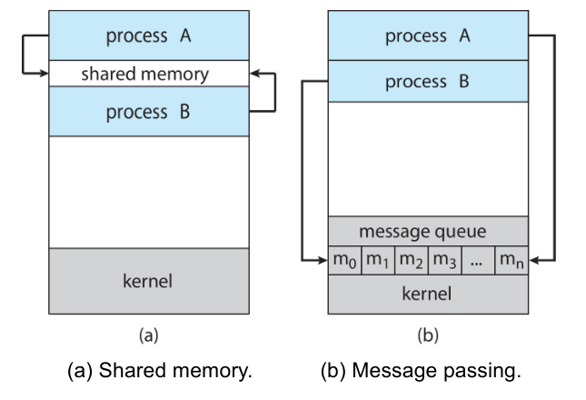
Shared Memory
This uses shared memory which requires communicating processes to establish a
region of shared memory.
Typically, a shared-memory region resides in the address space of the process
creating the shared-memory segment. Other processes that wish to communicated
using this shared-memory segment must attach it to their address space.
Consider a producer-consumer problem:
- A producer process produces information that is required by other processes.
- A consumer process reads and uses information is produced by the producer.
We create a buffer that can be filled by the producer and emptied by the
consumer. An unbounded buffer places no practical limit on the size of the
buffer. The bounded buffer assumes a fixed buffer size. In the second case,
the consumer must wait if buffer is empty and the producer must wait if buffer
is full.
#define BUFFER_SIZE 10

typedef struct {
    // ...
} item;

item buffer[BUFFER_SIZE];
int in = 0;
int out = 0;
The shared buffer is implemented as a circular array with two logical
pointers in and out.
The producer uses the following code to add items to the buffer:
item next_produced;

while (true) {
    /* Produce and item in next_produced */
    while (((in + 1) % BUFFER_SIZE) == out) {
        // do nothing while full.
    }

    buffer[in] = next_produced;
    in = (in + 1) % BUFFER_SIZE;
}
The consumer uses the following code to read items from the buffer:
item next_consumed;
while (true) {
    while (in == out) {
        /* do nothing when empty */
    }
    next_consumed = buffer[out];
    out = (out + 1) % BUFFER_SIZE;
    /* consume the item in next consumed */
}
This wouldn't work at the moment because buffer is just an array and the
processes would maintain separate copies. buffer needs to be "modified" to be
a region of shared memory. This scheme allows at most BUFFER_SIZE - 1 items in
the buffer at the same time.
Message Passing
Message padding provides a mechanism to allow processes to communicate and
synchronize their actions without sharing the same memory region.
It is particularly useful in a distributed environment, where the communicating
processes may reside on different computers connected by a network.
A message-passing facility provides at least two operations: send(message) and
receive(). If process P and Q want to communicate, a communication link
must exist between them.
Here are few options for the link:
- Direct or indirect communication
- Synchronous or asynchronous communication
- no buffering or automatic buffering.
Direct Communication
In direct communication, each process that wants to communicate must
explicitly name the recipient or sender of the communication.
A communication link in this scheme has the following properties:
- A link can be established between every pair of processes that want to
communicate. The processes need to know each other's identity to communicate.
- A link is associated with exactly two processes.
- Between each pair of processes, there exists exactly one link.
Indirect Communication
With indirect communication, the messages are sent to and received from
mailboxes or ports.
- A mailbox can be viewed abstractly as an object into which messages can be
placed by processes and from which messages can be removed.
- Each mailbox has unique identification.
- For example, POSIX message queues use an integer value to identify a mailbox.
In this scheme, a communication link has the following properties:
- A link is established between a pair of processes only if both members of the
pair have a shared mailbox.
- A mailbox may be associated with more than two processes.
- Between each pair of communicating processes, a number of different links may
exists, with each link corresponding to one mailbox.
Synchronous Communication
Communications between processes takes place through calls to send() and
receive() primitives.
There are different design options for implementing each primitive. Message
passing may be either blocking or non-blocking - also known as synchronous and
asynchrounous.
- Blocking send: After starting to send a message, the sending process is
blocked until the message is received by the receiving process or by the
mailbox.
- Non-blocking send: The sending process send the message and resumes
other operations.
- Blocking receive: After starting to wait for a message, the receiver is
blocked until a message is available.
- Non-blocking receive: The receiver is not blocked while it waits for the
message.
Buffering
Whether communication is direct or indirect, messages exchanged by communicating
processes reside in a temporary queue. Both the sender and receiver maintain a
queue.
- Zero capacity: The queue has a maximum length of zero.
- Bounded capacity: The queue has a finite length
n; thus at most n
messages can reside it in.
- Unbounded capacity: The queue's length is potentially infinite.
The zero-capacity case is sometimes referred to as a message system with no
buffering. The other cases are referred to as message systems with automatic
buffering.
Shared Memory vs Message Passing
Message passing:
Pros:
- Easy to setup and use.
- Can be used over networks and distributed environments.
Cons:
- Kernel needs to be involved in every distinct exchange of data.
- Is slow since messages need to be handled by the kernel.
Shared Memory:
Pros:
- Faster speeds since only required to establish a shared memory region.
- Most flexibility, you can access memory in any way the programmer likes.
Cons:
- More work for programmer since mechanisms needs to be explicitly coded.
- Less suitable for distributed environments - difficult to share memory.
Shared Memory Implementation
With POSIX , shared memory is implemented using memory-mapped file. The code is
based on the instruction here:
wikipedia
- Create a shared-memory object using the
shm_open system call.
- Once the object is created, the
ftruncate function is used to configure the
size of the object in bytes.
- The
mmap function maps a file to a memory section so that file operations
aren't needed.
POSIX Producer:
#include <stdio.h>
#include <stdlib.h>
#include <string.h>
#include <unistd.h>
#include <sys/shm.h>
#include <sys/stat.h>

int main() {
    const int SIZE = 4096; // the size (in bytes) of shared memory object
    const char *name = "OS"; // name of the shared memory object
    const char *message_0 = "Hello"; // strings written to shared memory
    const char *message_1 = "World"; // strings written to shared memory

    int shm_fd; // shared memory file descriptor
    void *ptr;  // pointer to shared memory object

    // Create the shared memory object
    shm_fd = shm_open(name, O_CREAT | O_RDWR, 0666);

    // configure the size of the shared memory object
    ftruncate(shm_fd, SIZE);

    // memory map the shared memory object
    // When the first parameter is set to 0, the kernel chooses the address at
    // which to create the mapping. This is the most portable method of
    // creating a new mapping.
    // The last parameter is the offset. When it is set to 0, the start of the
    // file corresponds to the start of the memory object.
    // Designed memory protection: PROT_WRITE means it may be written.
    // MAP_SHARED indicates that updates to the mapping are visible to other processes.
    ptr = mmap(0, SIZE, PROT_WRITE, MAP_SHARED, shm_fd, 0);

    // sprintf(): It generates a C string and places it in
    // the memory so that ptr points to it.
    sprintf(ptr, "%s", message_0);

    // Note the NULL character at the end of the string is not included.
    // strlen() returns the length of a string, excluding the NULL character
    // at the end of the string.
    ptr += strlen(message_0);

    sprintf(ptr, "%s", message_1);
    ptr += strlen(message_1);

    return 0;
}
POSIX Consumer:
#include <stdio.h>
#include <stdlib.h>
#include <fcntl.h>
#include <sys/shm.h>
#include <sys/stat.h>

int main() {
    const int SIZE = 4096; // the size (in bytes) of shared memory object
    const char *name = "OS"; // name of the shared memory object

    int shm_fd; // shared memory file descriptor
    void *ptr;  // pointer to shared memory object

    // open the shared memory object
    shm_fd = shm_open(name, O_RDONLY, 0666);

    // memory map the shared memory object
    // Designed memory protection: PROT_READ means it may be read.
    ptr = mmap(0, SIZE, PROT_READ, MAP_SHARED, shm_fd, 0);

    // read from the shared memory object
    printf("%s", (char *)ptr);

    // remove the shared memory object
    shm_unlink(name);

    return 0;
}
When compiling the above programs, you need to link the realtime extensions
library by adding -lrt to the compiling command.
You can use the following functions to work with shared memory:
shm_open()ftruncate()mmap()shm_unlink()
Pipe
Pipe is a type of message-passing interprocess communication method.
There are different types of pipes and each one type has different conditions
and implementations:
-
Unidirectional vs bidirectional: The flow of information is either in one
direction or both directions.
-
Half duplex vs full duplex: If information can flow in both directions,
can it flow in both ways at the same time?
-
Relationship: Does the pipe enforce a relationship between the processes
such as a parent-child relationship.
-
Network communication: Can a pipe be formed over a network or does it
have to reside on the same machine?
Unnamed Pipes (ordinary pipe)
Ordinary pipes allow two processes to communicate in a standard
producer-consumer fashion where the producer writes to one end of the pipe
called the write end and the consumer reads from the other end called the
read end.
Unnamed pipes are:
-
Unidirectional - allow only one-way communication. Two different pipes can be
used to communicate in both ways.
-
A parent-child relationship is required to create a pipe this way. Usually
a parent creates a pipe and uses it to communicate to the child process.
-
As ordinary pipes require a parent-child relationship, this forces the
communication to be on the same machine. That is, network communication is not
allowed.
Ordinary pipes on UNIX systems are created used the pipe(int fd[]) function.
Note, that the fd is used as the variable name as it stands for file
descriptor.
fd[0]: the read end of the pipe.fd[1]: the write end of the pipe.
On UNIX, pipes are just treated as a special type of file. Therefore, we can use
the regular write() and read() functions to write and read from these pipes.
For more details on this topic, you can see:
Analysing Pipe operating In C
Example
#include <sys/types.h>
#include <stdio.h>
#include <string.h>
#include <unistd.h>

#define BUFFER_SIZE 25
#define READ_END 0
#define WRITE_END 1

int main (int argc, char *argv[]) {
    char write_msg[BUFFER_SIZE] = "Greetings";
    char read_msg[BUFFER_SIZE];

    int fd[2];
    pid_t pid;

    if (pipe(fd) == -1) {
        fprintf(stderr, "pipe failed.\n");
        return 1;
    }

    pid = fork();

    if (pid < 0) {
        fprintf(stderr, "Fork failed.\n");
        return 1;
    }

    if (pid > 0) {
        /* close the unused end of the pipe */
        close(fd[READ_END]);

        write(fd[WRITE_END], write_msg, strlen(write_msg) + 1);

        close(fd[WRITE_END]);
    } else {
        close(fd[WRITE_END]);

        read(fd[READ_END], read_msg, BUFFER_SIZE);
        printf("read: %s\n", read_msg);

        close(fd[READ_END]);
    }

    return 0;
}
Named Pipes
Named pipes provide a much more powerful communication tool:
- Communication can be bidirectional.
- Communication is only half-duplex (one at a time).
- No parent-child relationship is required.
- Named pipes continue to exist after communicating processes haves terminated.
- Named pipes require that communicating processes reside on the same
machine.
Note: on MS Windows version of named pipe, full-duplex communication is allowed
and the communicating processes may reside on different machines.
Named pipes are referred to as FIFOs in UNIX systems. Once created, they appear
as files in the file system.
Named pipes are created on UNIX systems using the mkfifo() system call and
manipulated using the open(), read(), write() and close() system calls.
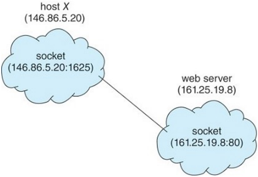
Socket
A socket refers to an endpoint for sending or receiving data across a
computer network. A pair of processes communicating over a network use a pair of
sockets (one for each process).
A socket is identified by an IP address concatenated with a port number, such as
185.139.135.65:5000.
Remote Procedure Call (RPC)
RPC is a special function call. The function (procedure) is called on the local
computer, but the function is executed on the remote computer. Once the function
execution is completed, the result is returned back to the local computer.
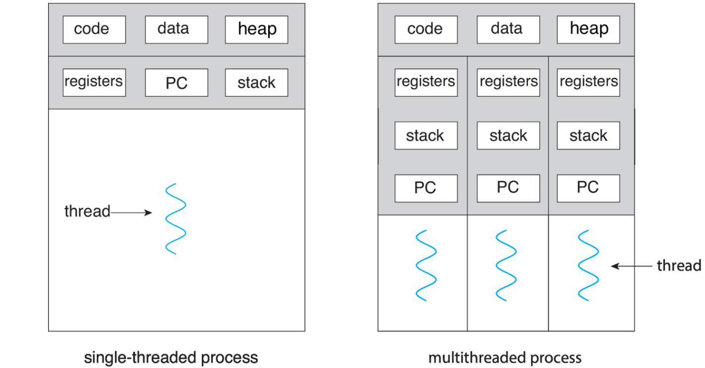
CH4: Threads and Concurrency
A thread is a basic unit of CPU utilization. It involves a thread ID, a
program counter (PC), a set of registers, and a stack.
It shares the following resources with other threads belonging to the same
process:
- Code/Text section
- Data section
- Heap section
- Other OS resources.
Benefits of Multithreaded Programming
-
Responsiveness: Multithreading an interaction application may allow a
program to continue running even if parts of it is blocked or is performing a
length operation.
-
Resource sharing: Threads share memory and the resources of the process
which they belong to. This makes it simpler to move resources between threads
compared to moving resources between processes.
-
Cost: Allocating memory and resources for process creation is costly.
Because threads share the resources of the process to which they belong, it is
more economical to create and context-switch threads.
-
Speed: The benefits of multithreaded programming can be even greater in a
multiprocessor architecture, where threads may run in parallel on different
processing processors.
Multicore Programming
Multithreaded programming provides a mechanism for more efficient use of
multiprocessor or multi-core systems.
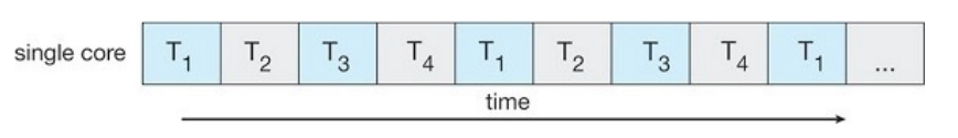
Consider an application with four threads. On a system with a single computing
core, concurrency merely means that the execution of the thread will be
interleaved over time.
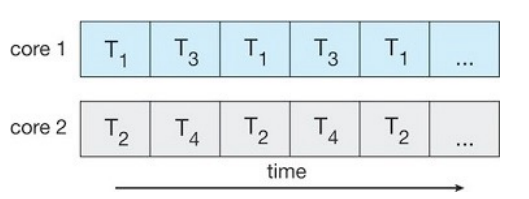
On a system with multiple cores, concurrency means that some threads can run
in parallel, because the system can assign a separate thread to each core.
Concurrency VS Parallelism
-
A concurrent system supports more than one task by allowing all tasks to
make progress using context-switches.
-
A parallel system can perform more than one task simultaneously. Multiple
instructions are being run at a given instant.
Therefore, it is possible to have concurrency without parallelism.
Challenges
Designing new programs that are multithreaded involves the following challenges:
-
Identifying tasks: Find tasks that can be done simultaneously.
-
Balance: Work between tasks should be similar to maximize speed.
-
Data splitting: Data access must be managed as now data may be accessed
by multiple tasks as the same time.
-
Data dependency: When one task depends on data from another, ensure that
the execution of the tasks is synchronized to accommodate the data dependency.
-
Testing and debugging: Testing and debugging multithreaded programs is
inherently more difficult.
User Level Threads VS Kernel Level Threads
Relationship
For the threads belonging to the same process, a relationship must exist between
user threads and kernel threads. There are three common ways of establishing
such as relationship:
- Many-to-one model
- One-to-one model
- Many-to-many model.
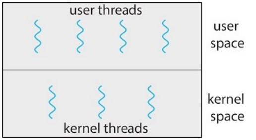
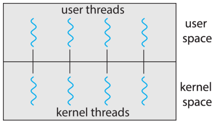
Many-to-One Model
This model maps multiple user-level threads to one kernel level thread.
-
A process is given a single kernel thread. There are multiple user-level
threads. Thread management is done by the thread library in the user space.
-
The entire process is blocked if one threads makes a blocking system call.
-
Multiple threads are unable to run in parallel on multicore systems.
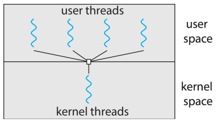
One-to-One Model
This model maps each user-level thread to one kernel level thread.
-
A process includes multiple kernel threads. There are multiple user-level
threads. Each user-level thread is mapped to one kernel thread.
-
It allows one thread to run when another thread makes a blocking system call.
-
It also allows multiple threads to run in parallel on multicore systems.
-
The drawback is that it creates a large number of kernel threads which may
worsen system performance.
Linux and Windows implement the one-to-one model.
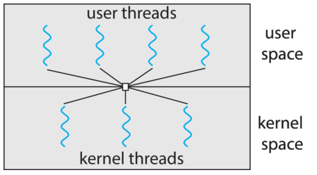
Many-to-Many Model
It multiplexes multiple user-level threads corresponding to a process to a
smaller or equal number of kernel threads corresponding to the same process.
-
The number of kernel threads may depends on a particular application or a
particular application.
-
An application may be allocated more kernel threads on a system with eight
processing cores than a system with four cores.
-
This means the developer can create as many threads as the like and the number
of kernel threads is not too large.
-
However, it is difficult to implement in practice and the increasing number of
processing cores appearing on most systems has reduces the importance of
limiting kernel threads.
Pthreads
Pthreads is a threads extension of the POSIX standard. This may be provided
as either a user-level or a kernel-level library. On Linux, it is implemented as
a kernel level library.
There are two strategies for creating multiple threads: asynchronous threading
and synchronous threading.
Asynchronous threading: Once the parent creates a child thread, the parent
resumes its execution, so that the parent and child execute concurrently and
independently of one another. Asynchronous threading is commonly used for
designing responsive user interfaces.
Synchronous threading: It occurs when the parent thread creates one or more
children and then must wait for all of its children to terminate before it
resumes. Typically, synchronous threading involves significant data sharing
among threads.
Example
Note: To compile programs using pthread.h, we need to include the -lpthread
argument to include the threading library when compiling our program.
#include <pthread.h>
#include <stdio.h>
#include <stdlib.h>

int sum;
void *runner(void *param) {
    int upper = atoi(param);
    sum = 0;
    for (int i = 1; i <= upper; i++) {
        sum += i;
    }
    pthread_exit(0);
}

int main(int argc, char *argv[]) {
    pthread_t tid;
    pthread_create(&tid, NULL, runner, argv[1]);
    pthread_join(tid, NULL);
    printf("sum = %d\n", sum);
    return 0;
}
Lifetime
Each C program starts with one thread, which corresponds to the main()
function. When the main() thread terminates, all threads belonging to the same
program will terminate. In general, a thread terminates if its parent thread
terminates.
Thread Count
Hyperthreading: Hyperthreading is Intel's simultaneous multithreading (SMT)
implementation used to improve parallelization of computations performed on x86
microprocessors. With hyperthreading, one physical core appears as two virtual
cores to the operating system, allowing concurrent scheduling of two threads per
core.
Thread Count: Theoretically, the total number of threads should be equal to
the number of cores of the system for optimal performance. On systems that
support hyperthreading, the number should be equal to twice the number of cores.
However, practically, the optimal number of threads vary on bunch of parameters
such as other running programs and the scheduling algorithm. Therefore, it is
best to experiment and find the best one.
Implicit Threading
Designing multithreaded programs involve many challenges, one way to address
these difficulties is to transfer the creation and management of threading from
application developers to compilers and run-time libraries. This strategy,
termed implicit threading, is an increasingly popular trend.
Implicit threading involves identifying tasks rather than threads. Once
identified, this is passed to the library which decides the optimal number of
threads to run. The library handles the thread creation and management.
The general idea behind a thread pool is to create a number of threads at
startup and place them into a pool, where they sit and wait for work. When the
OS receives a computation request, rather than creating a thread, it instead
submits the request to the thread pool and resumes, waiting for additional
requests.
Thread pools offer these benefits:
-
Servicing a request with an existing thread is often faster than waiting and
thereafter creating a thread.
-
A thread pool limits the number of threads that exists at any time point. This
is particularly important systems that cannot support large number of
concurrent threads.
-
Thread creation and management is transferred from application developers to
compilers and run-time libraries.
The numbers of threads in the pool can be set heuristically according to factors
such as:
- The number of CPUs in the system
- The amount of physical memory
- The expected number of concurrent client requests.
OpenMP
Open Multi-Processing (OpenMP) is an API for programs written in C, C++, or
FORTRAN, which provides support for parallel programming in shared-memory
environments.
OpenMP identifies parallel regions as blocks of code that may run in parallel.
Application developers insert compiler directives into their code at parallel
regions, and these directives instruct the OpenMP run-time library to execute
the region in parallel.
Example:
#include <stdlib.h>
#include <stdio.h>
#include <omp.h>

#define BUF_SIZE 1000000000

int main(int argc, char *argv[]) {

    int *a = malloc(BUF_SIZE * sizeof(int));
    int *b = malloc(BUF_SIZE * sizeof(int));
    int *c = malloc(BUF_SIZE * sizeof(int));

    // Initialize arrays
    #pragma omp parallel for
    for (int i = 0; i < BUF_SIZE; i++) {
        a[i] = 3;
        b[i] = 7;
        c[i] = 0;
    }

    #pragma omp parallel
    {
        printf("I am a parallel region.\n");
    }

    #pragma omp parallel for
    for (int i = 0; i < BUF_SIZE; i++) {
        c[i] = a[i] + b[i];
    }

    long long sum = 0;

    #pragma omp parallel for reduction(+:sum)
    for (int i = 0; i < BUF_SIZE; i++) {
        sum += c[i];
    }

    printf("total sum: %lld\n", sum);

    free(a);
    free(b);
    free(c);

    return EXIT_SUCCESS;
}
The output of which is:
I am a parallel region.
I am a parallel region.
I am a parallel region.
I am a parallel region.
I am a parallel region.
I am a parallel region.
I am a parallel region.
I am a parallel region.
I am a parallel region.
I am a parallel region.
I am a parallel region.
I am a parallel region.
I am a parallel region.
I am a parallel region.
I am a parallel region.
I am a parallel region.
total sum: 10000000000
Here we see that the string is printed 16 times. This is because the machine
that this code was run on has 16 threads. The for-loops are also executed
in parallel for initialization and summation.
In this code, the #pragma omp parallel for reduction(+:sum) directive tells
OpenMP to parallelize the loop and use the sum variable to accumulate the total
sum. Each thread will have its own local copy of sum, and at the end of the
parallel region, OpenMP will automatically sum up all these local copies into
the original sum variable. The + in reduction(+:sum) specifies that the
reduction operation is summation.
Here is my CPU while the process is running:
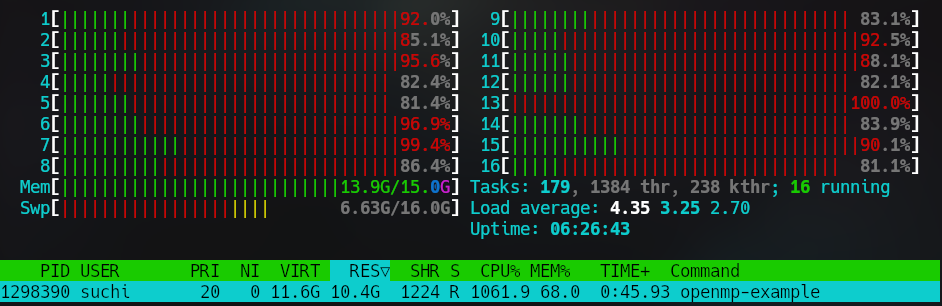
I wrote a single threaded version without using openmp and compared their
running times. The single threaded version took 22 seconds to execute where as
the openmp version only took 6 seconds. It was also clear that the single
threaded version was only using one core at any given time.
Here we clearly see that all my threads are being used. If you notice the code
doesn't have too many details about the parallelization - just a few lines about
the type of parallelization that we require.
CH5: CPU Scheduling
CPU scheduling is the basis of multiprogrammed operating systems. On modern
operating systems, it is kernel-level threads (no processes) that are in fact
being scheduled by the operating system. However, the terms "process scheduling"
and "thread scheduling" are often used interchangeably.
Typically, process execution alternates between two states:
- CPU burst: Where a process is mainly using the CPU.
- I/O burst: Where a process is performing I/O operations.
A process flips between CPU bursts and IO bursts. Eventually the final CPU
burst ends with a system request to terminate execution.
Although the durations of CPU bursts vary greatly from process to process.
However, most processes tend to have frequency curve similar to that shown in
the following figure:
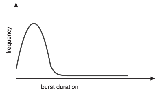
The curve is generally characterized as exponential or hyper exponential, with a
large number of short CPU bursts and a small number of long CPU bursts.
Whenever the CPU becomes idle, the operating system must select one of the
processes in the ready queue to be executed. The selection process is carried
out by the CPU scheduler, which selects a process from the processes in memory
that are ready to execute and allocates the CPU to that process.
The ready queue is a list of processes ready to be executed which is usually
records of process control blocks (PCBs) of the processes.
Preemptive VS Nonpreemptive
-
Nonpreemptive schedulers: once the CPU has been allocated to a process,
the process keeps the CPU until it releases it either by terminating or by
switching to the waiting state.
-
Preemptive schedulers: after the CPU has been allocated to a process, the
process could possibly lose the CPU before it terminates or switches to the
waiting state.
Dispatcher
The dispatcher is the module that gives control of the CPU's core to the
process selected by the CPU scheduler. This function involves the following
steps:
- switching context
- switching to user mode
- jumping to the proper location in the user program to restart the program.
The time it takes for the dispatcher to stop one process and start another
running is known as the dispatch latency.
Scheduling Algorithms
You'll find all the scheduling algorithms coded in C in the following
repository:
GitHub.
Evaluation Criteria For CPU Schedulers
Here are some typical criteria used to rank algorithms:
- CPU utilization: the percentage of the time when CPU is utilized.
- Throughput: the number of processes that complete their execution per unit
of time.
- Turnaround time: the interval from the time of submission of a process to
the time of completion.
- Waiting time: sum of the time spent waiting in the ready queue.
- Response time: the time from the submission of a process until the first
response is produced.
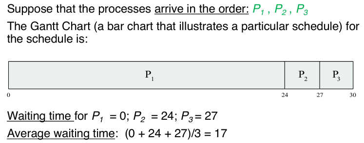
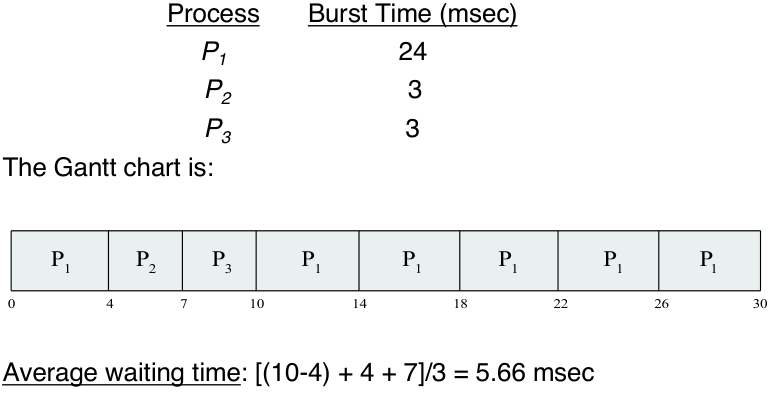
First-Come First-Served (FCFS)
The simplest CPU-scheduling algorithm is the first-come first-severed (FCFS)
scheduling algorithm. With this scheme, the process that requests the CPU first
is allocated first.
The implementation of the FCFS policy is easily managed with a FIFO queue. When
a process enters the ready queue, its PCB is linked onto the tail of the queue.
When the CPU is free, it is allocated to the process at the head of the queue.
The running process is then removed from the queue.
The negative with such an algorithm is that the average waiting time under the
FCFS policy is often quite long.
Suppose the processes arrive in the order: P1, P2, P3.
This algorithm suffers from the "convoy effect". The convoy effect is a
scheduling phenomenon in which a number of processes wait for one process to get
off a core, causing overall device and CPU utilization to be suboptimal.
Overview of FCFS:
- Simple implementation
- Nonpreemptive nature
- Long average waiting time
- Experiences convoy effect
- Bad for interactive systems.
Here is the algorithm written for a simulation of CPU scheduler:
Github FCFS
Shortest Job First (SJF)
The shortest-job-first (SJF) is an algorithm that schedules the job with the
shortest CPU burst first. When the CPU is available, it is assigned to the
process that has the smallest next CPU burst. If two processes have the same CPU
burst then FCFS scheduling is used to break the tie.
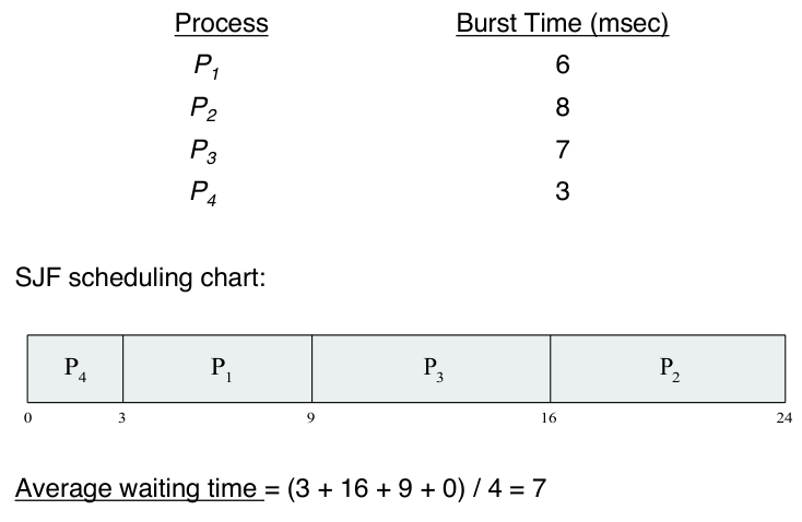
The SJF scheduling algorithm is provably optimal, in that it gives the minimum
average waiting time for a given set of processes.
Here is the algorithm written for a simulation of CPU scheduler:
Github Nonpreemptive SJF
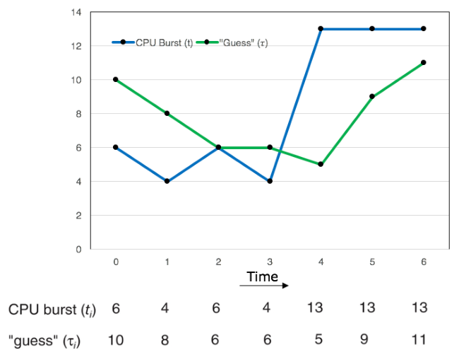
Predicting Next CPU Burst
However, we need to know the next CPU burst before we schedule algorithms based
on this. But, we can't know the CPU burst of a process before it is scheduled.
Therefore, we use a predicted CPU burst to schedule algorithms.
The following notations are used in the prediction:
- \(t_n\): the length of the current CPU burst.
- \(\tau_n\): the predicted value of the current CPU burst.
- \(\tau_{n+1}\): the predicted value for the next CPU burst.
- \(\alpha\): a tuning parameter \((0 \leq \alpha \leq 1)\), typically, \(\alpha = 1/2\).
The following equation can be used to predict the next CPU burst:
\[
\tau_{n+1} = \alpha t_n + (1 - \alpha)\tau_n
\]
This equation adds a fraction of the previous prediction and the previous CPU
burst to calculate the predicted CPU burst. The parameter \(\alpha\) controls
the relative weight of the previous CPU burst in our prediction. So, the highest
the value of \(\alpha\), the more we want \(t_n\) to affect our prediction.
The initial \(\tau_0\) can be defined as a constant or as an overall system
average.
Preemptive SJF
The SJF algorithm can be either preemptive or non-preemptive.
Consider a situation where a process arrives at the ready queue with a shorter
CPU burst when a process is currently running. If the scheduler considers
removing the current process and scheduling the new one then it is preemptive.
If the scheduler will always allow the process running to finish before
scheduling the next process then it is non-preemptive.
Here is an example:
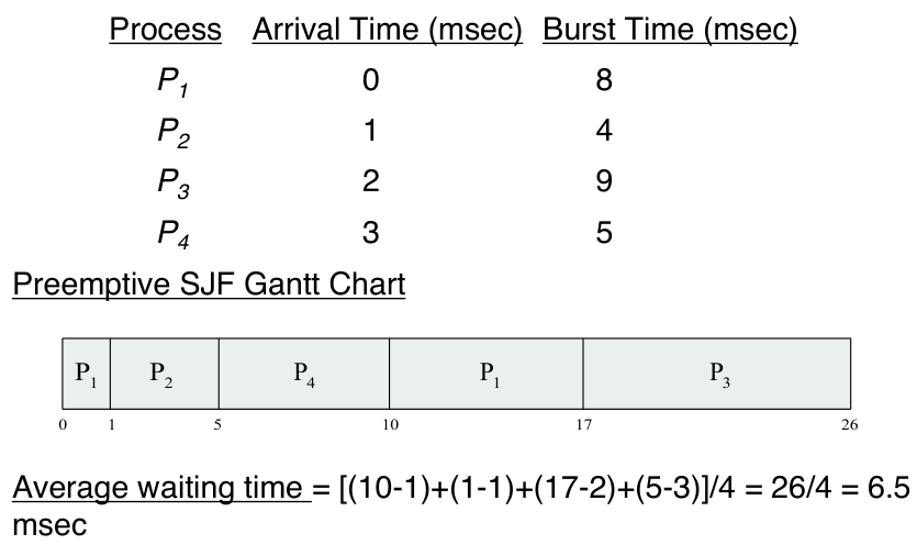
Here we see that process \(P_1\) was scheduled but when \(P_2\) arrived, it has
a shortest CPU burst than the remaining CPU burst of \(P_1\), and therefore
replace \(P_1\).
Here is the algorithm written for a simulation of CPU scheduler:
Github Preemptive SJF
Round Robin (RR)
The round-robin (RR) scheduling algorithm is similar to FCFS scheduling, but
preemption is added to enable the system to switch between processes.
Each process, when scheduled given a small unit of time, called a time
quantum or time slice that it can run for. Once the time quantum is done,
another process is scheduled. The ready queue is treated as a circular queue.
The CPU scheduler goes around the ready queue, allocating the CPU to each
process for a time interval of up to 1 time quantum.
If the CPU burst of the currently running process is longer than 1 time quantum,
the timer will go off and will cause an interrupt to the operating system. A
context switch will be executed, and the process will be put at the tail of
the ready queue. The CPU scheduler will select the next process in the ready
queue. Thus, the RR scheduling algorithm is thus preemptive.
Here is the algorithm written for a simulation of CPU scheduler:
Github Round Robin
The average waiting time is typically high in this policy.
Example:
The performance of the round robin algorithm depends heavily on the size of the
time quantum. If the time quantum is extremely large then the policy behaves the
same as the FCFS policy. In contract, if the time quantum is extremely small,
the policy can result in a large number of context switches.
The turnaround time also depends on the size of h time quantum. The
following figure shows the average turnaround time for a set of processes for a
given time quantum:
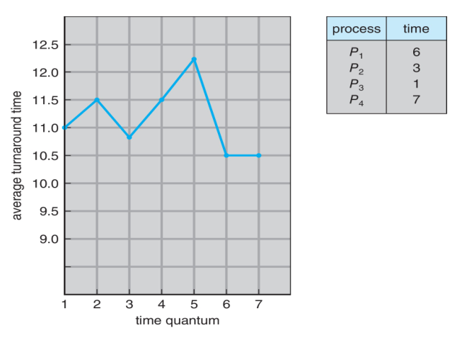
We can see that turnaround time does not necessarily improve as the time-quantum
size increases.
In general, the average turnaround time can be improved if most processes finish
their next CPU burst in a single time quantum. The time quantum should be large
compared with the context-switch time, but it should not be too large. A rule of
thumb is that 80 percent of the CPU bursts should be shorter than the time
quantum.
Priority Scheduling
A priority is associated with each process, and the CPU is allocated to the
process with the highest priority. Processes with equal priority are scheduled
in FCFS order.
In this course, we assume that a low number represents a high priority. However,
this is only a convention.

-
Priorities can be defined either internally or externally.
-
Internal priorities use some measurable quantity or quantities to compute the
priority of the process. Example, memory requirements, open files, etc.
-
External priorities are set by criteria outside the operating system. On
Linux you can use the nice command to change the priority of a process.
A major problem with priority scheduling algorithms is indefinite blocking
or starvation. This is when a low-priority task is never scheduled because
higher priority tasks keep showing up.
A solution to this problem is aging. This involves gradually increasing the
priority of the processes that wait in the system for a long time.
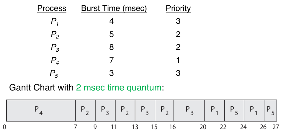
Priority Scheduling with Round-Robin
Priority scheduling can be combined with the round-robin scheduling so that the
system executes the highest-priority process using priority scheduling and runs
processes with the same priority using round-robin scheduling.
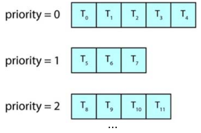
Multilevel Queue Scheduling
With priority scheduling, all processes may be placed in a single queue and the
scheduler selects the process with the highest priority to run. Depending on how
the queues are managed, an \(O(n)\) search may be necessary to determine the
highest-priority process.
In practice, it is often easier to have separate queues for each distinct
priority, which is known as a multilevel queue.
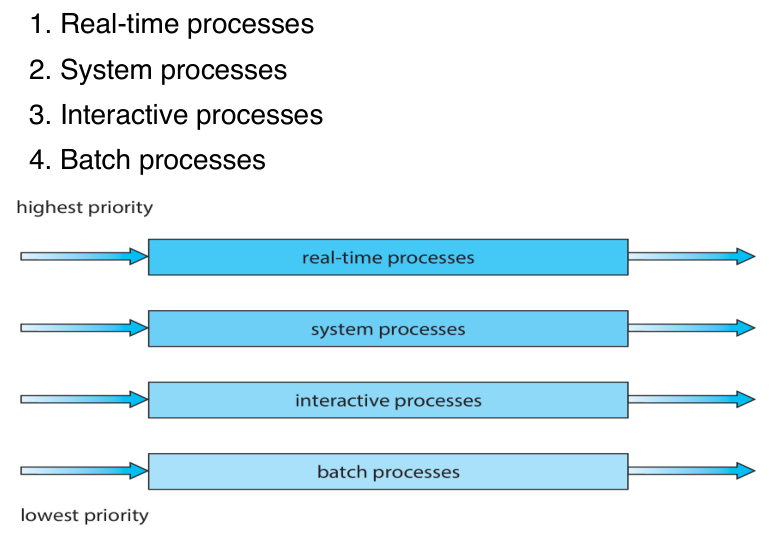
A multilevel queue could be used to achieve a flexible process scheduling. A
multilevel queue scheduling algorithm typically partitions processes into
several separate queues based on the process type. For example, separate queues
can be maintained for background and foreground processes.
Each queue could have its own scheduling algorithm. For example, the foreground
queue could be scheduled by an RR algorithm while the background queue could be
scheduled by FCFS algorithm.
Another possibility is to time-slice among the queues where each queue gets a
certain portion of the CPU time, which it can then schedule among its various
processes. For instance, in the foreground-background queue example the
foreground queue can be given 80 percent of the CPU time and the background
queue gets 20 percent of CPU time.
Feedback Based Scheduling
Normally, when the multilevel queue scheduling algorithm is used, processes are
permanently assigned to a queue when they enter the system. This setup has the
advantage of low scheduling overhead but it is inflexible.
The multilevel feedback queue scheduling algorithm, in contrast, allows a
process to move between queues. The idea is to separate processes according to
the characteristics of their CPU bursts.
If a process uses too too much CPU time, it will be moved to a lower-priority
queue. This scheme leaves I/O bound and interactive processes in the
higher-priority queues.
In addition, if a process that waits too long in a lower-priority queue may be
moved to a higher-priority queue. This is a form of aging prevents starvation.
For example, consider a multilevel feedback queue scheduler with three queues,
numbered from 0 to 2. The scheduler first executes all processes in queue 0.
Only when queue 0 is empty will it execute processes in queue 1. A process in
queue 1 will be preempted by a process arriving for queue 0. A process that
arrives for queue 1 will preempt processes in queue 2.
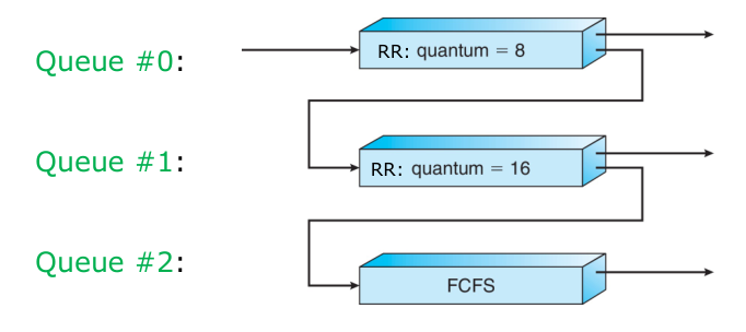
-
An entering process is put in queue 0.
- A process in queue 0 is given a time quantum of 8 milliseconds.
- If it does not finish within this time window, it is moved to the tail of
queue 1.
-
If queue 0 is empty, the process at the head of queue 1 is given a quantum of
16 milliseconds.
- If it does not complete within the time window, it it moved to tail of
queue 2.
- If a process arrives in queue 0 then a process is queue 1 is preempted.
-
If queue 0 and 1 are empty, the processes in queue 2 are run on an FCFS
basis.
- If a process arrives in queue 0 or 1, then a process is queue 2 is preempted.
-
To prevent starvation, a process that waits too long in a lower-priority
queue may gradually be moved to a higher-priority queue.
The definition of a multilevel feedback queue scheduler makes it the most
general CPU-scheduling algorithm. However, this also makes it the most complex
algorithm.
Thread Scheduling
On most modern operating systems, it is kernel-level threads (not processes)
that are being scheduled by the operating system.
For systems using many-to-one models, two steps are required to allocate the CPU
to a user-level thread:
-
Process contention scope (PCS): Locally, the threads belonging to the same
process are scheduled so that a user-level thread could be mapped to a
kernel-level thread.
-
System Contention Scope (SCS): Globally, kernel-level threads are
scheduled so that the CPU could be allocated to a kernel-level thread.
For systems using a one-to-one mode, such as Windows and Linux, only SCS is
required.
Multiple-Processor Scheduling
The scheduling algorithms we have discussed only talk about how to schedule
processes assuming a single processor. But most computers today have multiple
processing cores, how do we handle such situations?
-
Asymmetric Multiprocessing: A single processor, the master server,
handles all scheduling decisions, I/O processing, and other system activities.
The other processors only execute user code. This method is simple to
implement because only one processor accesses the system data structures,
reducing the need for data sharing. However, this potentially becomes a
bottleneck that could affect overall system performance.
-
Symmetric Multiprocessing (SMP): It is the standard scheme for a
multiprocessor system. Each processor is self-scheduling. Namely the scheduler
for each processor examine the ready queue and select a process to run.
With SMP, there are two possible strategies to organize the processes eligible
to be scheduled. Either we have a single ready queue or each processor is given
its own private ready queue.
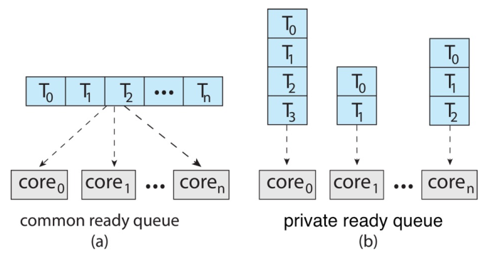
Since strategy (b) does not require any synchronization to access the queue, it
is the most common approach on systems supporting SMP.
Load Balancing
Load balancing attempts to keep the workload evenly distributed across all
processors in an SMP system. This is an important consideration to fully utilize
the benefits of having multiple processors.
Load balancing is typically necessary only on systems where each processor has
its own private ready queue of eligible processes to execute. On systems with a
common queue, load balancing is unnecessary.
There are two general approaches to load balancing: push migration and pull
migration.
-
Push Migration: a specific task periodically checks the load on each
processor; if it finds an imbalance, it evenly distributes the load by moving
processes from overloaded to idle (or less-busy) processors.
-
Pull Migration: in this case, an idle processor pulls a waiting process
from a busy processor.
Pull and push migration do not need to be mutually exclusive and are, in fact,
often implemented in parallel on load-balancing systems. For example, the Linux
process scheduler, Completely Fair Scheduler (CFS), implements both
techniques.
Processor Affinity
On most systems, each processor has its own cache memory. When a process has
been running on a specific processor the data most recently accessed by the
process populate the cache of the processor. As a result, successive memory
accesses by the process are often satisfied by cache memory.
If a process migrates to another processor, say, due to load balancing the
contents of the cache memory must be invalidates for the first processor, and
the cache for the second processor must be repopulated.
Because of the high cost of invalidating and repopulating cache, most operating
systems with SMP support try to avoid migrating a process from one processor to
another. This is known as processor affinity. A process has an affinity for
the processor on which it is currently running. There is an attempt to always
assign the same processor to a given processor.
Examples
Process scheduling in Linux:
-
Until Version 2.5: The Linux kernel ran a variation of the traditional
UNIX scheduling algorithm. This algorithm was not designed with SMP systems in
mind, it did not adequately support systems with multiple processors.
-
With Version 2.5: The scheduler was overhauled to include a schedulling
algorithm known as \(O(1)\) that run in constant time regardless of the number
of tasks in the system. This also provided increased support for SMP systems,
including processor affinity and load balancing between processors. This leads
to excellent performance on SMP systems but leads to poor response times for
interactive processes that are common on many desktop computer systems.
-
With Version 2.6 In release 2.6.23 of the kernel, the Completely Fair
Scheduler (CFS) became the default Linux scheduling algorithm.
Algorithm Evaluation
-
Deterministic Modeling: an evaluation method for scheduling algorithms.
This method takes a particular predetermined workload and generates the
performance of an algorithm under that workload. However, it requires exact
numbers for input and its answers only apply to those specific cases. These
methods can be used to indicate trends that can be analyzed.
-
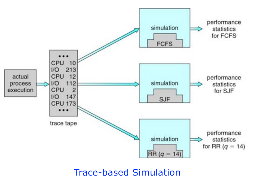
Simulations: Running a simulation involves programming a model of the
computer system. The data to drive the simulation can be generated in several
ways. The most common method uses a random-number generator that is programmed
to generate processes, CPU burst times, arrivals, departures, and so on.
- We can use trace files to monitoring the real systems and recording the
sequence of actual events. We then use this sequence to drive the
simulation.
Processes can be executed concurrently or in parallel. Context switch could be
carried out rapidly in order to provide concurrent execution. This means that
one process may only be partially completed before another process is
scheduled. Two different processes could be executed simultaneously on separate
processing cores.
We need to solve issues involving the integrity of data shared by several
processes.
Race Condition: A race condition occurs when two or more process can access
shared data and they try to change it at the same time. Because the process
scheduling algorithm can swap between processes at any time, you don't know the
order in which the processes will attempt to access the shared data. Therefore,
the result of the change in data is dependent on the thread scheduling
algorithm, i.e. both threads are "racing" to access/change the data.
Source For Race Condition
Here is a good YouTube Video that
explains race conditions and dead-locks.
Critical Section Problem
Consider a system with \(n\) processes \(\{p_0, p_1, \dots, p_{n-1}\}\). Each
process has a segment of code, called a critical section, which accesses and
updates data that is shared with at least one other process.
The important feature of the system is that, when one process is running in its
critical section, no other process is allowed to run in its critical section.
That is, no two processes run in their critical section at the same time.
The critical-section problem is about designing a protocol that the prcoesses
can use to synchronize their activity so as to cooperatively share data. With
this protocol, each process must request permission to enter its critical
section.
- Entry section: The section of code implementing the request.
- Exit section: The critical section may be follow by an exit section.
- Remainder section: the remaining code is the remainder section.
A solution must satisfy the following three requirements:
-
Mutual Exclusion: If process \(P_i\) is running in its critical section,
then no other processes can run in their critical sections.
-
Progress: If no process is running in its critical section and some
processes wish to enter their critical sections, then only those processes
that are not running in their remainder sections can participate in the
procedure of selecting a process to enter its critical section next, and
this selection cannot be postponed indefinitely.
-
Bounded Waiting: There exists a bound, or limit, on the number of times
that other processes are allowed to enter their critical sections after a
process has bade a request to enter its critical section and before that
request is granted.
Peterson's Solution
A software-based solution to the critical-section problem.
Important Note: However, because of the way modern computer architectures
perform basic machine-language instructions, there is no guarantee that
Peterson's solution will work correctly with such architectures. This is
primarily because to improve system performance, processors and/or compilers may
reorder read and write operations that have no dependencies.
Peterson's solution is restricted to two processes that alternate execution
between their critical sections and remainder sections. The processes are
numbered \(P_0\) and \(P_1\).
Peterson's solution requires the two processes to share two data items:
int turn;
boolean flag[2];
The variable turn indicates whose turn it is to enter its critical section.
That is, if turn == i, then process \(P_i\) is allowed to tun in its critical
section.
The array flag is used to indicate if a process is ready to enter its critical
section. If flag[i] is true, \(P_i\) is ready to enter its critical section.
while (true) {
    flag[i] = true;
    turn = j;
    while (flag[j] && turn == j) {
        // wait for j to finish
        ;
    }
    /* critical section */

    flag[i] = false;

    /* remainder section */
}
If both processes try to enter at the same time, turn will be set to both i
and j at roughly the same time. Only one of these assignments will last; the
other will occur but will be overwritten immediately. The eventual value of
turn determines which of the two processes is allowed to enter its critical
section first.
Hardware Synchronization
Hardware could be utilized to solve the critical-section problem. These include:
- Memory barriers
- Hardware instructions
- Atomic variables.
These solutions are generally complicated and inaccessible to application
programmers.
Mutex Locks
Mutex is short for "mutual exclusion". The operating system designers build
higher-level software tools to solve the critical-section problem. We use mutex
locks to protect critical sections and thus prevent race conditions. A process
must acquire the lock before entering a critical section; it releases the lock
when it exists the critical section.
The acquire() function acquires the lock, and the release() function
releases the lock, as illustrated in the following code.
while (true) {
    < acquire lock >
    critical section
    < release lock >
    remainder section
}
A mutex lock has a boolean variable available whose value indicates if the
lock is available or not. If the lock is available, a call to acquire()
succeeds, and the lock is considered unavailable. A process that attempts to
acquire an unavailable lock is blocked until the lock is released.
Calls to either acquire() or release() must be performed atomically (an
uninterruptible unit). This can be achieved via hardware support.
Spinlock: Mutex locks that just loop while they wait are also called
spinlocks. The process "spins" while waiting for the lock to become
available.
The advantage of spin locks is the they do not require a context switch. The
disadvantage is that they are wasting CPU cycles doing nothing. In certain
circumstances on multicore systems, spinlocks are in fact the preferred choice
for locking.
Mutex Locks In C
Here is an example of using mutex locks (from geeksforfeeks):
#include <pthread.h>
#include <stdio.h>
#include <stdlib.h>
#include <string.h>
#include <unistd.h>

pthread_t tid[2];
int counter;
pthread_mutex_t lock;

void* trythis(void* arg)
{
    pthread_mutex_lock(&lock);

    unsigned long i = 0;
    counter += 1;
    printf("\n Job %d has started\n", counter);

    for (i = 0; i < (0xFFFFFFFF); i++)
        ;

    printf("\n Job %d has finished\n", counter);

    pthread_mutex_unlock(&lock);

    return NULL;
}

int main(void)
{
    int i = 0;
    int error;

    if (pthread_mutex_init(&lock, NULL) != 0) {
        printf("\n mutex init has failed\n");
        return 1;
    }

    while (i < 2) {
        error = pthread_create(&(tid[i]), NULL, &trythis, NULL);
        if (error != 0)
            printf("\nThread can't be created :[%s]",
                strerror(error));
        i++;
    }

    pthread_join(tid[0], NULL);
    pthread_join(tid[1], NULL);
    pthread_mutex_destroy(&lock);

    return 0;
}
Semaphore
A semaphore is an integer variable that apart from initialization, is accessed
only through two indivisible (atomic) operations wait() and signal().
The wait and signal operations:
wait(S) {
    while (S <= 0)
        ;  // busy wait
    S--;
}

signal(S) {
    S++;
}
All modifications to the integer value of the semaphore in the wait() and
signal() operations must be executed atomically.
Semaphores In C
// C program to demonstrate working of Semaphores
#include <stdio.h>
#include <pthread.h>
#include <semaphore.h>
#include <unistd.h>

sem_t mutex;

void* thread(void* arg)
{
    //wait
    sem_wait(&mutex);
    printf("\nEntered..\n");

    //critical section
    sleep(4);

    //signal
    printf("\nJust Exiting...\n");
    sem_post(&mutex);
}


int main()
{
    sem_init(&mutex, 0, 1);
    pthread_t t1,t2;
    pthread_create(&t1,NULL,thread,NULL);
    sleep(2);
    pthread_create(&t2,NULL,thread,NULL);
    pthread_join(t1,NULL);
    pthread_join(t2,NULL);
    sem_destroy(&mutex);
    return 0;
}
Monitors
Although semaphores provide a convenient and effective mechanism for process
synchronization, using semaphores incorrectly can result in errors that are
difficult to detect.
Proposed by Hoare in 1974 and Brinch Hansen in 1975, monitors are a
language-specific synchronization construct. They provide a fundamental
guarantee that only one process may be in a monitor at any time.
Monitors must be implemented at the compiler/language level. The compiler must
ensure that the property is preserved. It is up to the compiler/language/system
to determine how mutual exclusion is implemented.
- Enters monitor
- Executes the critical section
- Leaves the critical section.
CH7: Synchronization Examples
The Dining Philosophers Problem
The Dining Philosophers Problem is an interesting and widely studied problem in
computer science, particularly in the realm of concurrency and resource
allocation.
Understanding the Situation
The problem is set around five philosophers who alternate between thinking and
eating. They share a circular table, each with their own designated chair. In
the center of the table lies a bowl of rice. Crucially, there are five single
chopsticks placed on the table. The philosophers, when deep in thought, do not
interact with each other.
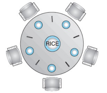
The Rules of Engagement
-
Eating and Thinking: Philosophers occasionally become hungry and attempt
to pick up the two chopsticks closest to them - one between them and their
left neighbor, and the other between them and their right neighbor.
-
Chopstick Handling: Each philosopher can only pick up one chopstick at a
time and cannot use a chopstick that's already in the hand of another
philosopher.
-
Eating Process: A philosopher eats only when they hold both chopsticks at
the same time, and upon finishing, they put down both chopsticks and resume
thinking.
The Technical Framework
From a programming perspective, the shared data is represented as semaphore
chopstick[5], with all semaphore elements initially set to 1. A philosopher
picks up a chopstick by performing a wait() operation on that semaphore and
releases the chopsticks using a signal() operation.
The routine of each philosopher can be described in the following pseudo C-code:
while (true) {
    wait(chopstick[i]);
    wait(chopstick[(i+1) % 5]);

    /* eat for a while */

    signal(chopstick[i]);
    signal(chopstick[(i+1) % 5]);

    /* think for awhile */
}
The Problem: Deadlock
The setup, as described, can lead to a deadlock. Imagine a scenario where
all five philosophers become hungry simultaneously and each grabs their left
chopstick. All semaphore elements (chopstick) would then be 0. As each
philosopher tries to grab their right chopstick, they find themselves unable to
proceed, leading to a deadlock where no philosopher can eat.
Solutions to Avoid Deadlock
-
Limiting the Number of Philosophers: One approach is to allow no more
than four philosophers at the table at any given time.
-
Critical Section for Chopsticks: Another solution is to allow a
philosopher to pick up both chopsticks only if both are available,
necessitating picking them up in a critical section.
-
Asymmetric Chopstick Pickup: A third solution proposes an asymmetric
method: odd-numbered philosophers first pick up their left chopstick, then
their right, while even-numbered philosophers do the opposite.
In summary, the Dining Philosophers Problem is more than a theoretical
conundrum. It serves as a valuable model for understanding complex issues in
concurrent programming and resource allocation, offering insights into solving
similar real-world problems.
POSIX Mutex Locks
Pthreads uses the pthread_mutex_t data types for mutex locks. A mutex is
created with the pthread_mutex_init() function. The first parameter is the
address of the mutex variable. By passing NULL as a second parameter, we
initialize the mutex with its default attributes.
#include <pthread.h>

pthread_mutex_t mutex;

/* create and initialize the mutex lock */
pthread_mutex_init(&mutex, NULL);
The mutex is acquired and released with pthread_mutex_lock() and
pthread_mutex_unlock() functions. If the mutex lock is unavailable, when
pthread_mutex_lock() is invoked, the called thread is block till the owner
invokes pthread_mutex_unlock().
/* acquire the mutex lock */
pthread_mutex_lock(&mutex);

/* critical section */

/* release the mutex lock */
pthread_mutex_unlock(&mutex);
When a mutex is not used any more, pthread_mutex_destroy() could be used to
eliminate the mutex.
pthread_mutex_destory(&mutex);
All pthread mutex functions return a value of 0 in the case of correct
operation; if an error occurs, these functions return a non-zero error code.
To compile a program involving pthread mutex lock, you can use the following
compiling command:
POSIX Semaphores
Semaphores are not a part of the POSIX standard and instead belong to the POSIX
SEM extension. POSIX specifies two types of semaphores: named and unnamed.
POSIX Named Semaphores
The function sem_open() is used to create and open a POSIX named semaphore:
#include <semaphore.h>

sem_t *sem;

/* create the semaphore and initialize it to 1 */
sem = sem_open("SEM", O_CREAT, 0666, 1);
- We are naming the semaphore
SEM.
- The
O_CREAT flag indicates that the semaphore will be created if it does not
exist.
- Additionally, the semaphore can be accessed via read and write (via the
parameter
0666) and is initialized to 1.
The advantage of named semaphores is that multiple unrelated processes can
easily use a common semaphore as a synchronization mechanism by simply referring
to the semaphore's name.
In POSIX, the wait() and signal() semaphore operations are implemented as
sem_wait() and sem_post(), respectively.
/* acquire the semaphore */
sem_wait(sem);

/* critical section */

/* release the semaphore */
sem_post(sem);
To destroy a named semaphore, you need to close the semaphore and thereafter
unlink it:
sem_close(sem);
sem_unlink("SEM");
POSIX Unnamed Semaphores
An unnamed semaphore is created and initialized using the sem_init() function,
which involves three parameters:
- The address of the semaphore variable
- A flag indicating the level of sharing
- The semaphore's initial value.
#include <semaphore.h>
sem_t sem;

/* create the semaphore and initialize it to 1 */
sem_init(&sem, 0, 1);
By passing 0 as the second parameter, we are indicating that this semaphore
can be shared only by threads belonging to the process that created the
semaphore, which is widely used in C programs involving semaphore. If we
supplied a nonzero value, we could allow the semaphore to be shared with
separate processes by placing it in a region of shared memory.
We acquire and release in the same way:
/* acquire the semaphore */
sem_wait(&sem);

/* critical section */

/* release the semaphore */
sem_post(&sem);
We can destroy the semaphore using the following:
Compiling For Semaphores
When you compile a program involving POSIX semaphore, you need to use the
following command:
Note, you will need to include -lrt if you are not using something after glibc
2.17 to include the real-time library.
CH8: Deadlocks
Deadlocks can be defined as a situation in which every process in a set of
processes is waiting for an event that can be cause only by another process in
the set.
-
Request: The process requests the resource. If the request cannot be
granted immediately (for example, if a mutex lock is currently held by
another process), then the requesting process must wait till it can acquire
the resource.
-
Use: The process can perform operations about the resource (for example, if
the resource is a mutex lock, the process can access its critical section).
-
Release: The process releases the resource.
Characterization
Deadlock could arise if four conditions are satisfied simultaneously.
-
Mutual Exclusion: Only one process can use a resource at a time.
-
Hold and Wait: A process holding at least one resource is waiting to
acquire additional resources held by other processes.
-
No Preemption: A resource can only be released voluntarily by the process
holding it, after that process has completed its task.
-
Circular Wait: There exists a set of waiting processes \(\{P_0, P_1,
\dots, P_n\}\) so that \(P_0\) is waiting for a resource that is held by
\(P_1\), \(P_1\) is waiting for a resource that is held by \(P_2, \dots,
P_{n–1}\) is waiting for a resource that is held by \(P_n\), and \(P_n\) is
waiting for a resource that is held by \(P_0\).
Deadlocks can be described more precisely using a directed graph called
resource-allocation graph.
This graph consists of a set of vertices \(V\) and a set of edges \(E\).
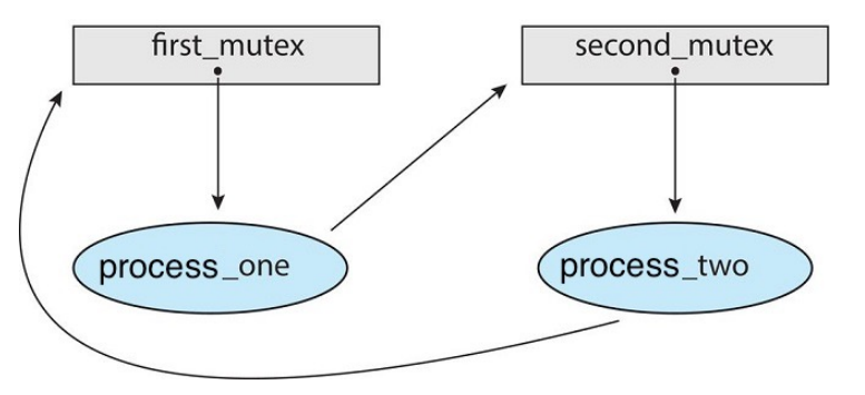
Given the definition of a resource-allocation graph, it can be shown
that, if the graph contains no cycles, then no process in the system is
deadlocked.
If the graph does contain a cycle, then a deadlock may exist.
-
If each resource type has exactly one instance, then a cycle implies that a
deadlock has occurred.
- If the cycle involves a set of resource types, each of which has only a
single instance, then a deadlock has occurred.
- Each process involved in the cycle is deadlocked.
- In this case, a cycle in the graph is both a necessary and a sufficient
condition for the existence of deadlock.
-
If each resource type has several instances, then a cycle does not necessarily
imply that a deadlock has occurred.
- In this case, a cycle in the graph is a necessary but not a sufficient
condition for the existence of deadlock.
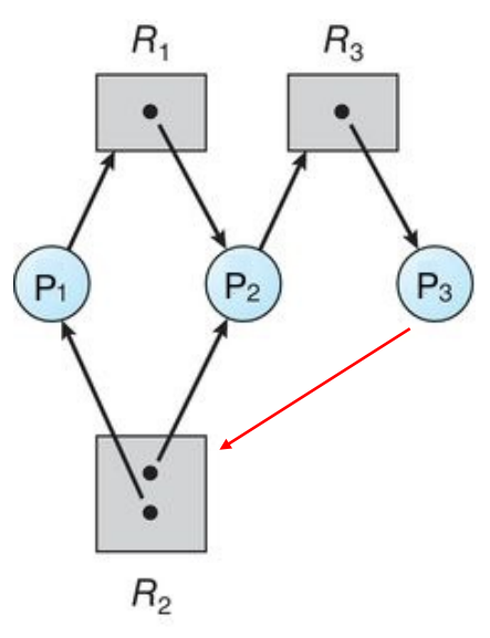
Solutions
Generally speaking, we can deal with the deadlock problem using one of the
following three methods:
-
Method 1: We can ignore the problem altogether and pretend that deadlocks
never occur in the system. If they happen rare enough it just might be better
to ignore them altogether.
-
Method 2: We can use a protocol to prevent or avoid deadlocks, ensuring that
the system will never enter a deadlock state.
-
Method 3: We can allow the system to enter a deadlocked state, detect it, and
recover.
Prevention
By ensuring that at least one of the four conditions for deadlocks cannot hold,
we can prevent the occurrence of a deadlock.
Mutual exclusion: Mutual exclusion is not required for shareable resources.
It must hold for non-shareable resources. In general, however, we cannot
prevent deadlocks by denying the mutual-exclusion condition because some
resources are intrinsically non-shareable.
Hold and Wait: To ensure that hold-and-wait never occurs, we must
guarantee that whenever a process requests a resource, it does not hold any
other resources.
-
All-then-execute: Require process to request and be allowed all its
resources before it begins execution.
-
None-then-request: Allow process to request resources only when the
process has none allocated to it. A process may request some resources and
use them. Before it can request any additional resources, it must release
all the resources that it is currently allocated.
This suffers from two disadvantages:
-
Low resource utilization: resources may be allocated but unused for a long
period. For example, a process may be allocated a mutex lock for its entire
execution, yet only require it for a short duration.
-
Starvation: A process that needs several popular resources may have to
wait indefinitely because at least one of the resources that it needs is
always allocated to some other process.
No Preemption: To ensure that this condition does not hold, we can use the
following protocol:
-
If a process that is holding some resources requests another resource that
cannot be immediately allocated to it, then all resources currently being held
are released.
-
Preempted resources are added to the list of resources for which the process
is waiting.
-
Process will be restarted only when it can regain its old resources, as well
as the new ones that it is requesting.
Circular Wait: Require that each process requests resources in an increasing
order of enumeration. That is, a process can initially request an instance of a
resource, say \(R_i\). After that, the process can request an instance of
resource \(R_j\) if and only if it has a higher number.
Avoidance
Deadlock avoidance involves requiring additional information on how resources
will be requested.
The simplest and most useful model requires that each process declares the
maximum number of instances of each resource type that may be needed.
In this scenario, a deadlock-avoidance algorithm dynamically examines the
resource allocation state to ensure that a circular-wait condition can never
exist.
When a process requests an available resource, the system must decide if
allocating the resource immediately leaves the system in a safe state. A system
is in a safe state only if there exists a safe sequence.
A sequence of processes, \(P_1, \dots, P_n\) is a safe sequence for the current
resource allocation state if, for each \(P_i\), the resource requests that
\(P_i\) might make can be satisfied by the currently available resources plus
the resources held by all \(P_j\) with \(j < i\).
There are two deadlock avoidance algorithms. For systems with single-instance of
each resource type we use "resource-allocation-graph algorithm". For systems
with multiple instances of each resources type we use "Banker's algorithm".
Resource Allocation Graph Algorithm
We introduce a new claim edge \(P_i \to R_j\) which indicates that process
\(P_j\) may request resource \(R_j\) at some time in the future. This is denoted
by a dashed-line. A claim edge is converted to a request edge when the process
requests the resource.
With this algorithm, resources must be claimed in advance in the system.
Now if a process requests a resource, we check if this could potentially form a
cycle. If yes, then we do not allow the process to access the resource even if
it is available. This is because a cycle puts the system into an unsafe state.
We only allow the process to access the resource once there is not longer the
opportunity for a cycle.
Detection
If each type of resource has only a single instance, then we can define a
deadlock-detection algorithm that uses a variant of the resource-allocation
graph, called a wait-for-graph.
We can obtain this graph from the resource-allocation graph by removing the
resource nodes and collapsing the appropriate edges. More precisely, an edge
from \(P_i\) to \(P_j\) in a wait-for graph implies that process \(P_i\) is waiting for process
\(P_j\) to release a resource that \(P_i\) needs. An edge \(P_i \to P_j\) exists in a wait-for
graph if and only if the corresponding resource-allocation graph contains two
edges \(P_i \to R_q\) and \(R_q \to P_j\) for some resource \(R_q\).
Here is an example of a resource-allocation graph being converted to a wait-for
graph:
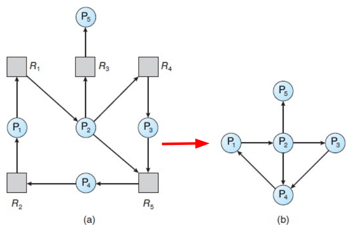
As before, a deadlock exists in the system if and only if the wait-for graph
contains a cycle. To detect deadlocks, the systems needs to maintain the
wait-for graph and periodically invoke an algorithm that searches for a cycle in
the graph.
Recovery
We have two options when we detect a deadlock in the system:
-
Aborting Processes: the first option is simply to abort one or more processes
to break the deadlock.
-
Resource Preemption: The other is to preempt some resources from one or more
of the deadlocked processes.
To eliminate deadlocks by aborting processes, we use one of two methods:
-
Abort all deadlocked processes. This method clearly will break the deadlock
cycle, but at a great expense. The deadlocked processes may have computed for
a long time, and the results of these partial computations must be discarded
and probably will have to be recomputed later.
-
Abort one process at a time until the deadlock cycle is eliminated. This
method incurs considerable over overhead, since after each process is aborted,
a deadlock-detection algorithm must be invoked to determine whether any
processes are still deadlocked.
Many factors are involved in the termination of a process - we try to incur the
minimum cost:
- What the priority of the process is.
- How long the process has computed and how much longer the process will
compute.
- How many and what types of resources the process has used.
- How many more resources the process needs in order to complete.
To eliminate deadlocks by resource preemption, we successively preempt some
resources from processes and give these resources to other processes until the
deadlock cycle is broken.
If preemption is required to deal with deadlocks, then three issues need to be
addressed:
-
Selecting a victim: which resources and which processes are to be preempted?
As in process termination, we must determine the order of preemption to
minimize cost.
-
Rollback: If we preempt a resource from a process, what should be done with
that process? The simplest solution is a total rollback: abort the process
and restart it.
-
Starvation: How do we ensure that starvation will not occur? That is, how can
we guarantee that resources will not always be preempted from the same
process?
CH9: Main Memory
There are a couple of rules that the operating system enforces on the processes
to ensure the proper functioning of the system.
One solution to this problem is to have a separate memory space for each
process. To separate memory space, we need to have a range of legal addresses
that a process may access and to ensure that the process can access only its
legal addresses. We can provide this protection using two registers, usually a
base register and a limit register.
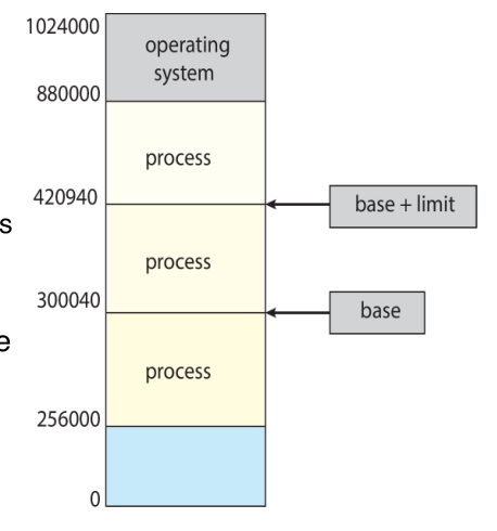
Logical VS Physical Address
Logical Address: The address from the perspective of the user program. It is
also known as virtual address. The corresponding memory space is called logical
memory space. A user program only uses logical addresses and thinks that the
corresponding process runs in a memory space with the address range of 0 to max.
Physical Address The real address for each storage unit in main memory. The
corresponding memory space is called physical memory space. The logical
addresses must be mapped to physical address before the data in main memory can
be accessed. We use a relocation register (same as base register) to accomplish
the mapping.
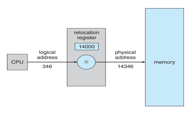
Contiguous Memory Allocation
With contiguous memory allocation, each process is contained in a single section
of memory, which is typically next to the section containing the next process.
One of the simplest methods of allocating memory is to assign variable-sized
sections of memory to processes. With this variable-section scheme, the
operating system keeps a table indicating which parts of memory are available
and which are occupied.
A hole in memory is just a region of memory that is not used.
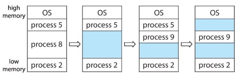
When a process is loaded into memory, the OS needs to find a proper hole to
allocate enough memory to the processes.
Dynamic Storage Allocation: It is a memory allocation method used to satisfy
a request of size \(n\) with a list of free holes.
- First fit: Allocate the first hole that is big enough.
- Best fit: Allocate the smallest hold that is big enough.
- Worst fit: Allocate the largest hole.
Simulations have shown that both first fit and best fit are better than worst
fit in terms of memory utilization but neither is "clearly better" than the
other, but first fit is generally faster.
External Fragmentation: This is when there is enough total memory space to
satisfy a request, but the available spaces are not contiguous.
Internal Fragmentation: If a system employs a fixed size allocation then if
a process requests 40 Kb but is given 64 Kb then internal fragmentation exists.
Paging
Paging is a memory-management scheme that permits a processes' physical address
space to be non-contiguous. Paging avoids the external fragmentation problem.
The basic method of implementing paging involves:
- Breaking physical memory into fixed-sized blocks called frames.
- Breaking logical memory into same size blocks called pages.
Then we map each page to a frame.
When a process is to be executed, its pages are loaded into available memory
frames. The page number is used as an index into a per-process page table.
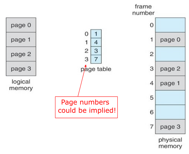
Every logical address can be divided into two parts: a page number (p) and a
page offset (d).
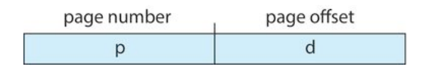
To translate a logical address to a physical address:
- Extract the page number \(p\) and use it as an index into the page table.
- Extract the corresponding frame number \(f\) from the page table.
- Replace the page number \(p\) in the logical address with the frame number
\(f\).
As the offset \(d\) does not change, it is not replaced, and the frame number
and offset now form the physical address.
The page size is defined by the hardware. It is usually determined by the
processor architecture. The size of a page is a power of 2 bytes, typically
varying between 4KB and 1 GB per page, depending on the computer architecture.
If the size of the logical address space is \(2^m\) bytes, a page size is
\(2^n\) bytes, and the computer is byte-addressable, then the high-order (m-n)
bits of a logical address correspond to the page number, and whatever is left in
the logical address (the n low-order bits) designate the page offset.
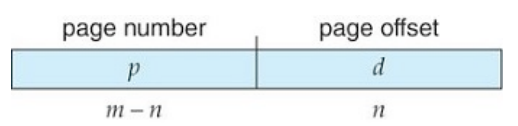
Conversion from logical address to physical address example:
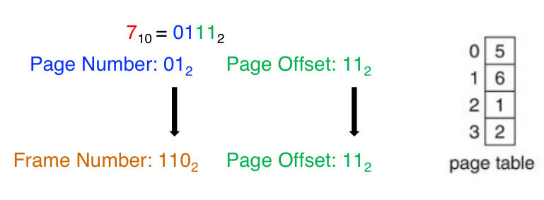
When using a paging scheme, we have no external fragmentation, any free frame
can be allocated to a process that needs it. However, we may have some internal
fragmentation.
The allocation information is generally kept in a single system-wide data
structure called a frame table.
Most modern computer systems support a large logical address space. In such
environments, the page table itself becomes very large.
Hierarchical Paging
To solve the problem of page tables becoming very large, we use a two-level
paging algorithm, in which the page table itself is also paged.
Swapping
We can use some of our external storage such as a hard drive or SSD as pretend
memory. After a process is loaded into memory, the process can be swapped out
temporarily out of memory to a backing store and then bought back into memory
for continued execution.
Swapping enables the possibility that the total address space of all processes
exceeds the real physical memory of the system.
Standard Swapping involves moving an entire process between main memory and
a backing store. When a process is swapped to the backing store, the operating
system must also maintain metadata for processes that have been swapped out, so
they can be restored when they are swapped back into memory.
This method was used int traditional UNIX systems, but it is generally no longer
used in contemporary operating systems, because the amount of time required to
move the entire process between memory and the backing storage is prohibitive.
Paged Swapping: involves swapping pages of a processes rather than the
entire process. This strategy still allows physical memory to be
oversubscribed, but does not incur the cost of swapping entire processes.
In fact, the term "swapping" now generally refers to "standard swapping", and
"paging" refers to "swapping with paging".
A page out operation moves a page from memory to the backing store and the
reverse is known as a page in.
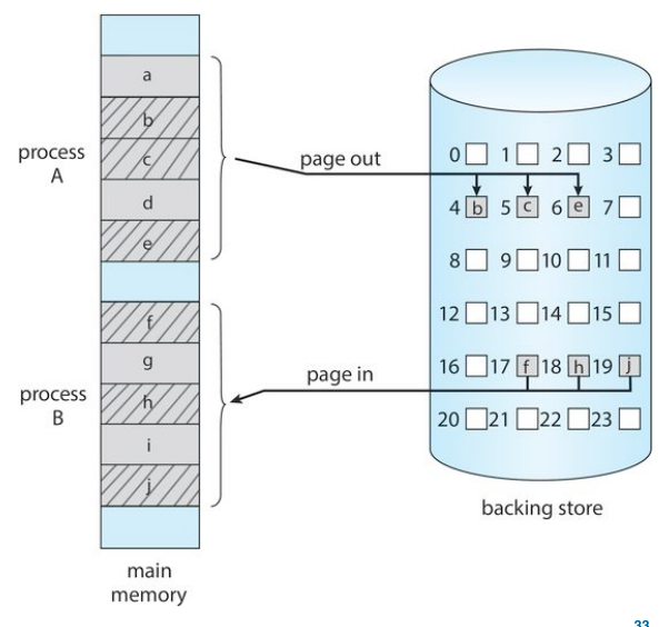
CH10: Virtual Memory
Demand Paging
When a program is loaded into memory, two methods could be used.
-
Method 1: Load the entire program in physical memory at program execution
time. However, we may not initially need the entire program in memory.
-
Method 2: Load pages only when they are needed. This technique is known as
demand paging and is commonly used in virtual memory systems. With
demand-paged virtual memory, pages are loaded only when they are demanded
during program execution.
With demand paging, while a process is executing, some pages will be in memory,
and some will be in secondary storage. Thus, we need some form of hardware
support to distinguish these two cases.
We can add a bit to identify if a page is valid. When the bit is set of valid,
the corresponding page is in memory. When the bit is set of invalid, the page is
currently in secondary storage.
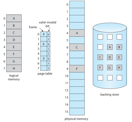
When a process tries to access a page that has not been brought into memory, it
will cause a page fault, resulting in a trap to the OS. Here is the procedure
used to access physical memory when a page fault is generated:
- Extract the address from the current instruction.
- Use page table to check whether the corresponding page has been loaded. If
valid-invalid bit is 'invalid', a trap is generated.
- Find a free frame in physical memory.
- Move the desired page into the newly allocated frame.
- Modify the page table to indicate that the page is now in memory.
- Restart the instruction that was interrupted by the trap. The process can now
access the page as if it had always been in memory.
Demand paging can significantly affect the performance of a computer system.
Assume the memory access time, denoted as \(ma\), is \(200\) nanoseconds.
Let \(p\) be the probability of a page fault. We would expect \(p\) to be close
to zero. That is, we could expect to have only a few page faults.
The effective access time can be calculated using the following equation:
\[
\text{effective access time } = (1-p) * ma + p * \text{ page fault time}
\]
Page Replacement
In the case that a page fault occurs and there is no free frame, the OS has to
use one of the "page replacement" algorithms to
- Find a victim frame
- Move the victim frame to secondary storage
- Move the page that caused the page fault into the freed frame.
Note that in this case, two page transfers are required. This situation
effectively doubles the page-fault service time and increases the effective
access time accordingly.
We can evaluate an algorithm by running it with a particular series of memory
references and computing the number of page faults. This series of memory
references are called a reference string. We can generate references string
artificially, or we can trace a given system and record the address of each
memory reference.
FIFO Page Replacement
A FIFO replacement algorithm associates with each page the time when the page
was brought into memory. When a page must be replaced, the oldest page is
chosen.
OPT Page Replacement
The optimal page replacement algorithm (OPT) should replace the page that will
not be used for the longest period of time. Use of this page-replacement
algorithm guarantees the lowest possible page-fault probability for a fixed
number of frames.
Unfortunately, the optimal page replacement algorithm is difficult to implement
because it requires knowledge about the future (how the memory will be
accessed). As a result, the optimal algorithm is used mainly for comparison
purposes.
LRU Page Replacement
The Least Recently Used replacement associates with each page the time of that
page's last use. When page must be replaced, LRU chooses the page that has not
been used for the longest period of time.
Allocation of Frames
The number of frames that should be allocated to a program initially depends on
a couple of factors. There are a few options:
Equal Allocation: The easiest way to allocate \(m\) frames to \(n\) processes
is to give each one an equal share, \(m/n\) frames.
Proportional Allocation: The available memory is allocated to each process
according to its size.
Let the size of the virtual memory for process \(p_i\) be \(s_i\), and define
\(S = \sum s_i\). If the total number of available frames is \(m\), we allocate
\(a_i\) frames to process \(p_i\), where \(a_i\) is approximately \((s_i/S) *
m\).
CH11: Mass Storage Systems
Secondary storage for modern computers is provided by hard disk drives (HDD) or
nonvolatile memory (NVM) devices.
Hard Disk Drives
- Each drive has multiple platters*.
- Each platter looks like a CD.
- Two surfaces of a platter are covered with a magnetic material.
- We store information by recoding it magnetically on the platters.
- We read information by detecting the magnetic pattern on the platters.
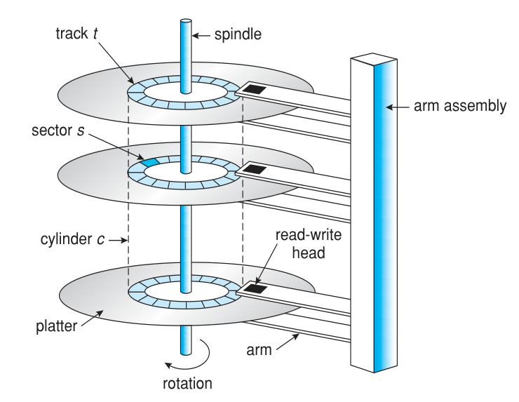
The surface of a platter is logically divided into circular tracks, which are
subdivided into sectors.
Each sector has a fixed size and is the smallest unit of transfer. The sector
size was commonly 512 bytes until around 2010. At that point manufacturers
started migrating to 4KB sectors.
The set of tracks at a given arm position make up a cylinder. A disk drive
motor spins at high speeds.
There are number of parameters that determine how fast the data on HDDs can be
accessed.
- Seek Time is the time that it takes a disk arm to position itself over the
required track.
- Rotational Delay is the time that it takes the desired sector to position
itself under the read/write head.
- Access Time = Seek Time + Rotational Delay
- Transfer Time = Access Time + Time To Read Data
- Transfer Rate gives us the rate at which data can be read from the disk.
Nonvolatile Memory Devices (NVM)
Nonvolatile memory decides are normally based on flash memory technology.
- Solid State Disk: It is frequently used in a disk-drive-like container,
leading to SSD.
- USB Drive: It can be embedded in a device with a USB interface, leading to USB
drive.
- Surface-mounted Storage: It is also surface-mounted onto motherboards as the
main storage in devices like smartphones.
On the positive side:
- NVM devices can be more reliable than HDDs because they have no moving parts.
- NVM devices can be faster because it does not use the mechanical read-write
head to read/write data.
- In addition, they consume less power.
On the negative side:
- They are more expensive per megabyte than traditional hard disks and have less
capacity than the larger hard disks.
- NVM devices deteriorate with every write, and stop working after approximately
100,000 writes.
Connection Methods
A secondary storage device is attached to a computer by the system bus or an I/O
bus. Several kinds of buses are available, including: Advanced technology
attachment (ATA), Serial ATA (SATA), eSATA, Serial Attached SCSI (SAS),
Universal serial bus (USB), Fiber Channel (FC).
Because NVM devices are much faster than HDDs the industry created a special,
fast interface for NVM devices called NVM express (NVMe).
Address Mapping
Storage devices are addressed as large one-dimensional arrays of logical blocks,
where the logical block is the smallest unit of transfer.
For HDD, each logical block is mapped to a physical sector. By using this
mapping on an HDD, we can convert a logical block number into an old-style disk
address that consists of a cylinder number, a track number within that cylinder,
and a sector number within that track.
For NVM devices, mapping can be done in a similar manner.
Scheduling
We can use on of the HDD scheduling algorithms to minimize access time and
maximize transfer rate.
FCFS Scheduling
The simplest form of disk scheduling is FCFS. This algorithm is intrinsically
fair, but generally does not provide the fastest service.
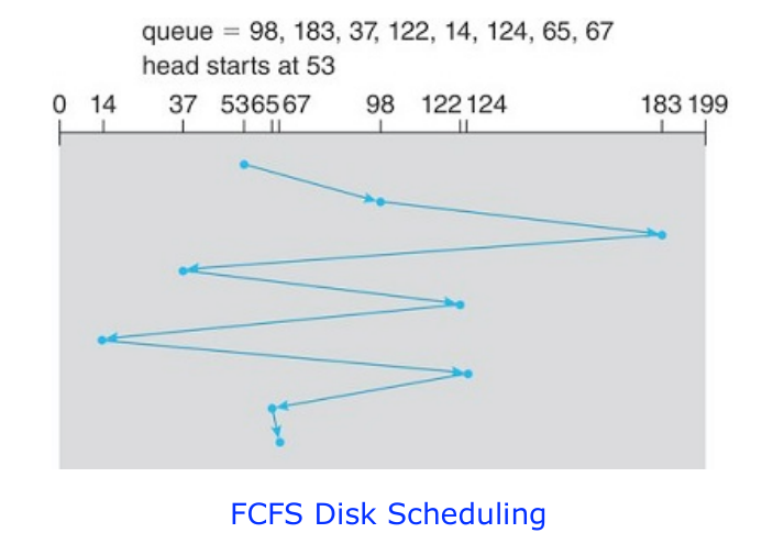
SCAN Scheduling
With the SCAN algorithm the disk arm starts at one end of the disk and moves
toward the other end, servicing requests as it reaches each cylinder, until it
gets to the other end of the disk. At the other end, the direction of the head
movement is reversed, and the servicing continues.
The SCAN algorithm is sometimes called the elevator algorithm, since the
disk arm behaves like an elevator in a building, first servicing all the
requests going up and then reversing to service requests the other way.
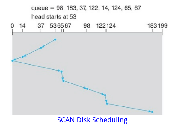
C-SCAN Scheduling
Since after completing a scan of the disk, the heaviest density of requests is
at the other end of the disk, C-SCAN starts the next scan at the start again.
Circular SCAN (C-SCAN) scheduling is a variant of SCAN designed to provide a
more uniform wait time. When the head reaches the other end, it immediately
returns to the beginning of the disk without servicing any requests on the
return trip.
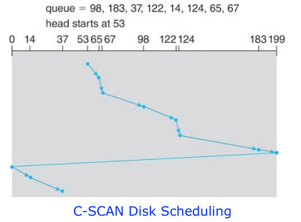
NVM Scheduling
The disk-scheduling algorithms apply to mechanical platter-based storage like
HDDs. The algorithms focus primarily on minimizing the amount of movement of
the disk head.
NVM devices do not contain moving disk heads and commonly use a simple FCFS
policy.
As we have seem, I/O can occur sequentially or randomly.
-
Sequential access is good for mechanical devices like HDD and tape because
the data to be read or written is close to the read/write head.
-
Random-access I/O, which is measured in input/output operations per second
(IOPS), causes more HDD disk movement. Naturally, random access I/O is much
faster on NVM.